Home
Search
Up
Reference Manuals
Return
Users Manual for Program MPLOT
Table of contents
Introduction
Flow chart
Command line options
Pulldown menus
Mouse button control
Post processing
Input data commands which controls post processing
Calculate different ride comfort assessments
Designing higher order filters
Plotting
Introduction
Input data at the lowest input data level
Input data valid at level DIAGRAM
Input data valid at level PAGE
Input data valid at level MAIN
All plotting commands in alphabetical order
Examples
Introduction
Program MPLOT reads result files written in MPdat format,
having the file extension .id or
.mp.
Program MPLOT has two main functions:
- Post-processing
Algebraic operations, filtering, statistical evaluations and different transformations
can be made.
All available post-processing commands are documented under
Input data commands which controls post processing.
- Plotting
Two- and three- dimensional plots of scalars and vectors.
The user has possibility to select results from many different idents by adding
the name of the ident enclosed in parenthesis after the name of the variable.
All available plot-processing commands are documented under
Input data commands which controls plotting.
Some notes on the input data reading:
- Input data is read in free format, valid separators between the input data are
<space>, <comma>, <tab>, <equal sign> or <carriage return>.
The commands are understood both in lower and upper case letters.
- Lines starting with a #-sign will be treated as commentary lines.
- Lines starting with a !-sign will be sent as a command to the UNIX system.
- In the description of the input data commands in this manual,
certain simplifications have been made in order to reduce the text volume
in this document.
The simplifications are implemented according to the same method as listed in
the user manual for the CALC program.
The simplifications are:
- Words enclosed between grave accents ` `
The program expects to read a valid string, which provides a valid
main- or sub- command.
An error will occur if integer or real are read.
- Words enclosed between a grave accent and an acute accent ` '
The program expects to read a string which must be a variable
previously defined in the input data.
An error will occur if integer or real are read.
- Words without accents
The program expects to read data constants which comprise integer or real.
An error will occur if the character is read.
- Words which begin with a grave accent `
At this stage, the program expects to read a character string or a data constant.
If a string is read, the program will seek the variable which
has been assigned that name and will store the address to the variable.
If a data constant is read, the value will be stored directly in the memory.
- Words which begin with signs and a grave accent +-`
At this stage, the program accepts reading a variable or a constant.
The variable or constant can have up to two preceding signs minus and/or plus.
- Words which begin with signs and a grave accent in parenthesis (+-`)
At this stage, the program accepts reading a variable or a constant.
The variable or constant can have up to two preceding signs minus and/or plus.
The parentheses imply that if a variable is read, its value will not be updated.
Program CALC will only use the value of the variable at time=tstart.
Reference Manuals
Mplot menu
Flow chart
The flow of data in GENSYS is carried out as follows:
Activity 1
The results from the calculation activity TSIM, FRESP, MODAL or QUASI are stored
in MPdat-format on an output data file named '\$ident.id'.
The variables stored in the *.id-file are
defined in the CALC-command s_var.
Activity 2
Program MPLOT copies the contents of file '\$ident.id' into the files '\$ident.mp' and '\$ident.mp2',
because it is much faster to read and write in direct access files.
The files '\$ident.mp' and '\$ident.mp2' are also working as a memory for program
MPLOT, holding all new vectors and scalars generated in the post processing
commands.
In the command line arguments -save_mp
and -no_save_mp the user can control
if the files '\$ident.mp' and '\$ident.mp2' shall be saved or not after the
MPLOT activity.
Activity 3
Plots can be created by reading result data files from several idents at the same time.
If *.mp- and *.mp2- files do exist they will be read and plotted,
but if they do not exist program MPLOT will use the *.id-files.
Reference Manuals
Mplot menu
Command line options
When launching program MPLOT the user can supply a number of command line options.
The user can put his or hers favorite options in a file named gen_conf.
File gen_conf is primarily searched in the local working directory.
If file gen_conf not can be found in the local working directory,
program MPLOT searches for file .gen_conf in the users home-directory.
If no file can be found locally or in the \$HOME-directory, program MPLOT
will read the file \$gensys/bin/gen_conf.
Following command line options are understood:
| -addarg | = | Prompt for more arguments before calculation starts |
| -no_addarg | = | Do not prompt for more arguments |
| -debug | = | Don't remove temporary work files |
| -h or -help | = | Print this help information |
| | | |
| -interactive | = | Run MPLOT in interactive mode (please see further information under Description of pulldown menus). |
| -no_interactive | = | Run MPLOT in batch mode. |
| | | |
| -pri | = | Print all results on printer \$LPDEST=lp1 |
| -pri_graphics | = | Print graphical results. |
| -pri_resu | = | Print result-textfile *.resu. |
| -pri_textfiles | = | Print all other result-textfiles from program MPLOT. |
| -no_pri | = | Do not print any results at all.(Default) |
| -no_pri_graphics | = | Do not print graphical results. |
| -no_pri_resu | = | Do not print result-textfile *.resu. |
| -no_pri_textfiles | = | Do not print all other result-textfiles from program MPLOT. |
| | | |
| -q_sys batfile | = | Write plot commands into file batfile, if batfile=stdout write plot commands to standard output |
| | | |
| -res_1600x1200 | = | Resolution 1600x1200 pixels |
| -res_1280x1024 | = | Resolution 1280x1024 pixels |
| -res_1024x768 | = | Resolution 1024x768 pixels |
| -res_800x600 | = | Resolution 800x600 pixels |
| | | |
| -save_mp | = | Save workspace in file \$ident.mp |
| -save_graphics | = | Save graphical results (Default) |
| -save_resu | = | Save the result-textfile *.resu (Default) |
| -save_textfiles | = | Save all other result-textfiles from program MPLOT (Default) |
| -no_save_mp | = | Do not save workspace (Default) |
| -no_save_graphics | = | Do not save graphical results. |
| -no_save_resu | = | Do not save the result-textfile *.resu. |
| -no_save_textfiles | = | not save all other result-textfiles from program MPLOT. |
| | | |
| -use_MPfile | = | If an ident is stored in a file *.mp, read the file without questions |
| -no_use_MPfile | = | If an ident is stored in a file *.mp, remove the file |
| -ask_use_MPfile | = | If an ident is stored in a file *.mp, prompt the user if the file shall be read or not |
| | | |
| arg(1) | = | Input data file |
| arg(2) | = | Ident |
If not input data file and/or ident has been given among the command line options
script MPLOT will prompt the user for these items.
Reference Manuals
Mplot menu
Description of pulldown menus
If program MPLOT is started with the -interactive command line option.
The following pulldown menu will appear at the top of the window:
File
Post
Draw
Help
Reload
New
Edit
Pulldown menu File
| Open MPdat-file ... |
Opens a popup-menu for selection of a MPdat-file.
If a MPdat-file not is opened the user will be promoted for a MPdat-file
each time a new curve or point is selected. |
| Close MPdat-file |
Closes current MPdat-file. |
| Idents in time order |
Creates a list of all idents in current directory in time order. |
| Idents alphabetic |
Creates a list of all idents in alphabetic order. |
| Read mplotf-file ... |
Open and read a *.mplotf-file.
The diagrams are read and saved into the memory of the program.
The diagrams can be plotted by clicking on "Draw" + "Open_saved_page". |
| Print ... |
Opens a popup printer-menu, the user can select different graphic output
formats and if the results shall be send to printer or file. |
| Calculator ... |
Opens a popup-window in where numerical calculations can be done. |
| Command ... |
Manually write a command to the program MPLOT. |
| Import ... |
Import variables from columns read from external ASCII-file. |
| Export ... |
Export variables and scalars to a plain ASCII-file. |
| MPdat contents short |
Creates a list of all variables and scalars in opened MPdat-file.
Writes only a short list containing min-, max-, start- and end- values. |
| MPdat contents long |
Creates a list of all variables and scalars in opened MPdat-file.
Writes a full dump of all values for all variables in opened MPdat-file. |
| MPdat contents matlab |
Creates a list of all variables and scalars in opened MPdat-file.
Writes a full dump of all values for all variables in opened MPdat-file,
in a format readable for matlab. |
| Save plots and exit |
Stops the execution of program MPLOT.
Before program MPLOT quits the user has the possibility to store all created MPLOT-commands in an external mplotf-file. |
| Exit |
Stops program MPLOT, without storing MPLOT-commands. |
Pulldown menu Post
| filt ... |
Filtering of variables in time-domain
according to the command filt. |
| fourier ... |
Translates a variable to or from frequency domain
according to the command fourier. |
| ftwz ... |
Calculation of Ride Index Wz
according to the command ftwz. |
| func ... |
Algebraic postprocessing of variables
according to the command func. |
| stat ... |
Calculation of statistical properties
according to the command stat . |
| transt ... |
Filtering of time-domain variables in frequency domain
according to the command transt . |
| transf ... |
Filtering of frequency-domain variables in frequency domain
according to the command transf . |
Pulldown menu Draw
| Curve from current ident |
Opens a popup-window with a list of all curves in opened MPdat-file.
If no MPdat-file is opened, the user will be promted to select a MPdat-file first. |
| Curve from other idents |
Opens a popup-window where the user can select both ident and variable. |
| Scalar from current ident |
Opens a popup-window with a list of all scalars in opened MPdat-file.
If no MPdat-file is opened, the user will be promted to select a MPdat-file first. |
| Diagram # |
Opens a popup-window for selection of diagram number.
If the user changes current diagram number, further plotting will
be directed to the new diagram number. |
| Clear page |
Clears the contents of current page. |
| Reset scale factor |
Reset the view scale factor, if it has been modified with the mouse buttons. |
Pushbutton Edit
opens current page for editing.
Pushbutton Reload
rereads and reloads current page after editing.
(N.B. Current file must be saved before it can be reread.)
Pushbutton New
creates a new page.
The textfields to the right of the Edit-pushbutton shows current coordinate when mouse button #2 is pressed.
The radiobuttons to the right of the textfields, shows the number of current page.
Reference Manuals
Mplot menu
Mouse button control
In the interactive version of program MPLOT
| Btn #1 | Zoom in the picture by pressing and at the same time drag the mouse upwards in the window. |
| Btn #2 | Show current coordinate of the pointer.
The coordinates are written in the two text fields up in the pulldown menu. |
| Btn #3 | Panning in the window. |
| Wheel | Zoom by rotating the mouse wheel. |
| Wheel+CTRL | Pressing the CTRL-button at the same time, makes the zooming to go faster. |
Post processing
Input data commands which controls post processing
In Mplot there are a number of commands which create new curves and scalars.
This section was previously referred to as DYNPOST, but is today an integrated
part in Mplot.
The various mplot commands and the DYNPOST commands can be combined
today.
Input data for these commands are read in free format. Two principles
govern input of the input data:
- Alt 1)
first a main command is read, and directly after the main command
all input data are read in a long row.
- Alt 2)
first a main command is read, thereafter the input data is read by
subcommands.
The two input methods can also be combined, e.g. the user can begin with the method 1)
and then change to method 2), and vice versa.
When an input data variable is required "Iname" the user can choose to read the variable
from an other ident if he put the name of the ident directly after the name and
enclosed in parenthesis ex. "Iname(ident)"
The following post-processing commands are available at level MAIN in Mplot:
(the list begins with a brief summary)
| CREATE_CURVE | = | Directive to create a curve in the memory |
| CREATE_SCALAR | = | Directive to create a scalar in the memory |
| CATALO | = | Directive to inspect the content in the memory |
| CATFIL | = | Define the name of the output-file for command CATALO |
| DELETE_CURVE | = | Directive to delete a curve from the memory |
| DELETE_SCALAR | = | Directive to delete a scalar from the memory |
| ELSE | = | Precedes an else-block |
| ELSEIF_THEN | = | Precedes an elseif_then-block |
| ENDIF | = | Ends an if_then-block |
| EQDIST | = | Directive to generate equidistance time steps |
| FILT | = | Directive for filtration in time domain |
| FOURIER | = | Directive for Fourier transformation |
| FTWZ | = | Directive for FFT-transformation and Wz-calculation |
| FUNC | = | Directive to execute mathematical operations |
| IF_THEN | = | Define the beginning of an if_then-block |
| INSERT | = | Redirects input reading from another input file |
| IN_SUBSTRUCT | = | Directive which inserts a sub-structure |
| LOOP | = | Define the beginning of a loop-block |
| NO_WARNING | = | Directive which suppresses warning texts |
| NTABLE | = | Number of columns to be written in the *.resu-file. |
| PRINT | = | Directive to print results on ASCII-files |
| STAT | = | Directive for statistical analysis |
| STAT2 | = | Directive for 3-dimensional statistical analysis |
| SUBSTRUCT | = | Directive for defining substructures |
| TRANS | = | Filtering of a time domain variable in frequency domain |
| TRANSF | = | Filtering of a frequency domain variable in frequency domain |
| TRANST | = | As directive TRANS, but with argument Tsname |
| UNTIL | = | Define the end of a loop-block began in command LOOP |
| WZ_AFRESP | = | Calculation of Wz from a variable frequency domain |
Reference Manuals
Mplot menu
CREATE_CURVE, cc_func, input(*)
Command which creates new curves in current ident.
Command CREATE_CURVE have the following sub-commands:
cc_type = `append_sngl`
Adds new points to a new or existing vector in the memory.
create_curve append_sngl vname, tname, v_dim, values
| vname | = |
Name of the new or existing vector. If the vector is already
stored in memory, the values will be appended to the vector vname,
otherwise a new vector will be created in memory. |
| tname | = |
Vector vname:s default x-axis. When the plotting of a vname
in mplot and the x-axis is not specified, this vector will be
used as the x-variable. Tname must be stored in
memory before this command can be given, or tname must be assigned
the same name as the vname. If tname is not specified,
tname will be set to vname. |
| v_dim | = |
The dimension of the vector, which shall be placed in parentheses.
As default v_dim will be set the value 'blank'. |
| values | = |
Values which will be read into the vector. The input will be
ended when a new valid command is read. If the name of a scalar is read,
the value of the scalar be given to the vector. |
cc_type = `file_vpair_free`
Creates two vectors in the memory.
Command 'file_vpair_free' reads value-pairs from an external file.
If a line in the external file 'file' begins with the letter #
it will be regarded as a comment.
create_curve file_vpair_free tname, vname, t_dim, v_dim, format, file
| tname | = |
Name of the new X-vector.
The values of the vector will be read from the first column
in 'file'.
The file 'file' will be read according to the format defined in
'format'. |
| vname | = |
Name of the new Y-vector.
The values of the vector will be read from the second column
in 'file'.
The file 'file' will be read according to the format defined in
'format'. |
| t_dim | = |
The dimension of the X-vector.
The dimension shall be placed inside parentheses.
As default t_dim will be set the value 'blank'. |
| v_dim | = |
The dimension of the Y-vector.
The dimension shall be placed inside parentheses.
As default v_dim will be set the value 'blank'. |
| format | = |
The columns in file 'file' are read in free format.
The syntax of the character string format is as follows:
'(a,x,a,x)'
In the example above column 1 and 3 will be read from file 'file',
and column 2 and 4 will be skipped over.
The letter 'a' marks a column that shall be read,
and the letter 'x' marks a column that shall be skipped over.
In the example above program MPLOT expects to read a file containing
four columns.
If the file contains of only two columns, the second variable will
not be read and program MPLOT will then set all values in
vector vname to zero.
If the file contains of more than four columns, program MPLOT will
only read column one and three and all other columns will be
skipped over. |
| file | = |
The name of the file from which the vectors shall be read from.
If a line in the file begins with the letter #,
it will be regarded as a comment and all values on that line
will not be read. |
cc_type = `linear_increasing`
Creates a new vector in the memory, linearly increasing from vstart.
create_curve linear_increasing vname, vstart, vincr, npoints, v_dim
| vname | = |
Name of the new vector. |
| vstart | = |
Start value for the new vector. |
| vincr | = |
Increment between two consecutive values in vname. |
| npoints | = |
Number of points in vname. |
| v_dim | = |
The dimension of the vector, which shall be placed in parentheses.
As default v_dim will be set the value 'blank'. |
cc_type = `new_sngl`
Creates a new vector in the memory.
create_curve new_sngl vname, tname, v_dim, values
| vname | = |
Name of the new vector. |
| tname | = |
Vector vname:s default x-axis. When the plotting of a vname
in mplot and the x-axis is not specified, this vector will be
used as the x-variable. Tname must be stored in
memory before this command can be given, or tname must be assigned
the same name as the vname. If tname is not specified,
tname will be set to vname. |
| v_dim | = |
The dimension of the vector, which shall be placed in parentheses.
As default v_dim will be set the value 'blank'. |
| values | = |
Values which will be read into the vector. The input will be
ended when a new valid command is read. If the name of a scalar is read,
the value of the scalar be given to the vector. |
cc_type = `truncate`
Truncates an existing vector into a new vector.
create_curve truncate new_yvar new_xvar old_yvar old_xvar +-`tstart +-`tstop
| new_yvar | = |
Name of the new shorter vector. |
| new_xvar | = |
Name of the new shorter x-variable for new_yvar. |
| old_yvar | = |
Name of the existing vector. |
| old_xvar | = |
Name of the existing x-vector. |
| tstart | = |
X-value in old_xvar from where new_yvar and new_xvar will start.
|
| tstart | = |
X-value in old_xvar from where new_yvar and new_xvar will stop.
|
CREATE_SCALAR, cs_func, input(*)
Directive to create a new scalar in current ident.
TOC:
cs_type = `curve_first`
Creates a scalar in memory, which is the first value in a variable.
This command is redundant, please use create_scalar curve_interp instead.
create_scalar curve_first pname= vname
| pname | = | Name of the new scalar. |
| vname | = | Variable from which the first value shall be picked. |
cs_type = `curve_interp`
Creates a scalar in memory, interpolated from a variable.
create_scalar curve_interp pname= vname tval tname
| pname | = | Name of the new scalar. |
| vname | = | Variable from which the value shall be interpolated. |
| tval | = | Input X-value. |
| tname | = | Name of the X-variable. If undefined the default X-variable will be used. |
cs_type = `curve_last`
Creates a scalar in memory, which is the last value in a variable.
create_scalar curve_last pname= vname
| pname | = | Name of the new scalar. |
| vname | = | Variable from which the last value shall be picked. |
cs_type = `curve_sum`
Creates a scalar in memory, which is the sum of all the points of a variable.
create_scalar curve_sum pname= vname
| pname | = | Name of the new scalar. |
| vname | = | Variable from which all values shall be summed. |
cs_type = `curve_vmax`
Creates a scalar in the memory, which is the maximum value of a variable.
create_scalar curve_vmax pname= vname
| pname | = | Name of the new scalar. |
| vname | = | Variable from which the maximum value shall be picked. |
cs_type = `curve_vmax_x`
Creates a scalar in the memory, containing the X-value of the default X-axis, when the max value of vname was reached.
(After a simulation the default X-axis are "time" for all variables)
Scalar pname can be used in command create_scalar curve_interp
to find values of other variables that occurs at the same time as when vname reaches its maximum value.
create_scalar curve_vmax_x pname= vname
| pname | = | Name of the new scalar. |
| vname | = | Variable where the max value shall be searched in. |
cs_type = `curve_vmin`
Creates a scalar in the memory, which is the minimum value of a variable.
create_scalar curve_vmin pname= vname
| pname | = | Name of the new scalar. |
| vname | = | Variable from which the minimum value shall be picked. |
cs_type = `curve_zero`
Creates scalars in the memory,
containing all X-values for which variable vname is zero.
create_scalar curve_zero pname= vname
| pname | = | Basename of the new scalars. Command curve_zero adds the extension .z1 .z2 .z3 etc. for each time vname passes zero. |
| vname | = | The variable from where the zeros are read. |
cs_type = `new`
Creates a new scalar in memory.
create_scalar new pname= pvalue p_dim
| pname | = | Name of the new scalar. |
| pvalue | = | Numerical value of the scalar. |
| p_dim | = | The dimension of the scalar, which shall be placed in parentheses.
As default v_dim will be set the value 'blank'. |
CATALO= cat_type
Directive to inspect the contents of current ident.
The output is written to file defined in directive CATFIL below.
| cat_type | = |
Selects different type of prints, cat_type can be given one of the following
character string:
| "vectors" | = | Prints the vectors(variables) stored in memory |
| "points" | = | Prints the scalars stored in memory |
| "both" | = | Prints both vectors and scalars |
|
CATFIL= file-name
Define the name of the file to which the CATALO-output above will be written.
If the file-name is " " or "no", the output will be written to standard output.
The default value of file-name is "\$ident.cata".
DELETE_CURVE, pname
Directive to delete a vector in current ident.
| pname | = | Name of the vector which shall be deleted. |
DELETE_SCALAR, pname
Directive to delete a scalar in current ident.
| pname | = | Name of the scalar which shall be deleted. |
ELSE
The ELSE statement is used when coding an IF_THEN-else decision statement.
The keyword precedes an else-block, defined to be all the statements after the ELSE-statement up to,
but not including the corresponding ENDIF-statement.
ENDIF
The command ENDIF concludes the statement IF_THEN.
EQDIST, Iname, EQname, EQtime
Directive to generate curves with equidistant time steps.
| Iname | = | Name of the input variable. |
| EQname | = | Name of the output variable. If omitted Eqname will be set to 'EQ'+Iname. |
| EQtime | = | Name of the output variable's time variable. If omitted EQtime will be set to 'EQTIME'. |
FILT, Type, Num, Iname, Fname, Tname
Directive to filtrate in time domain. The command requires
that the input variable has equidistant time steps.
| Type | = | Type of filter, see table below. |
| Num | = | Numerical input data value, see table below. |
| Iname | = | Name of the input variable. |
| Fname | = | Name of the output variable. If omitted Tname will be set to 'F'+Iname. |
| Tname | = | Name of the time axis. If omitted the default x-variable for Iname will be used. |
| Type | Num | Function |
|---|
| DELAY | t_delay |
Delay Iname the amount t_delay.
A positive delay means that the curve is
shifted to a later point in time.
Program MPLOT fills the beginning of the variable with zeros.
If t_delay is not a multiple of the time step in Iname's
default time variable,
program MPLOT will interpolate the values
in variable Fname linearly, so that the two curves Iname and Fname
will have the same default time variable.
If variable Iname contains high frequency components this
interpolation can act as a low pass filtering effect. |
| DERIV | n/a | Derivation of the input variable Iname with regard to Tname. |
| INTEG | beg_value | Integration of the input variable Iname with regard to Tname.
Num defines the initial value of the integral. |
| HPASS1 | fo | First order high pass filter.
In the beginning, the output variable Fname will have the same
value as Iname as initial value. |
| HPASS1_0 | fo | First order high pass filter.
In the beginning, the output variable Fname will have the value=0
as initial value, regardless of the value of the input variable. |
| HPASS2 | fo,zeta | Second order high pass filter.
In the beginning, the output variable Fname will have the same
value as Iname as initial value. |
| HPASS2_0 | fo,zeta | Second order high pass filter.
In the beginning, the output variable Fname will have the value=0
as initial value, regardless of the value of the input variable. |
| LPASS1 | fo | First order low pass filter.
In the beginning, the output variable Fname will have the same
value as Iname as initial value. |
| LPASS1_0 | fo | First order low pass filter.
In the beginning, the output variable Fname will have the value=0
as initial value, regardless of the value of the input variable. |
| LPASS2 | fo,zeta | Second order low pass filter.
In the beginning, the output variable Fname will have the same
initial value as Iname.
"fo" defines the cut-off frequency of the filter and "zeta" defines
the fraction of critical damping of the filter. |
| LPASS2_0 | fo,zeta | Second order low pass filter.
In the beginning, the output variable Fname will have the value=0
as initial value, regardless of the value of the input variable.
"fo" defines the cut-off frequency of the filter and "zeta" defines
the fraction of critical damping of the filter. |
| MAX_ABS | t_incr | Sliding absolute max value calculation.
Filter MAX_ABS selects the value with biggest magnitude in window t_incr.
T_incr has the same dimension as variable "Tname".
If number of values in window t_incr is less than 1(one), MPLOT will write a warning message and no filtration is possible.
The window works as a fifo-memory (first in first out),
why "Fname" will be shifted in time relative to "Iname".
N.B. The sliding max_abs-value will adopt its value from one of the values in the window.
No extra- or interpolation will take place on the borders of window t_incr. |
| MAX_SIGN | t_incr | Sliding max value calculation.
Filter MAX_SIGN selects the largest value in window t_incr.
T_incr has the same dimension as variable "Tname".
If number of values in window t_incr is less than 1(one), MPLOT will write a warning message and no filtration is possible.
The window works as a fifo-memory (first in first out),
why "Fname" will be shifted in time relative to "Iname".
N.B. The sliding max_sign-value will adopt its value from one of the values in the window.
No extra- or interpolation will take place on the borders of window t_incr. |
| MEAN | t_incr | Sliding mean value calculation.
The size of the window which is used in the calculation
of the sliding mean value is defined in the variable t_incr.
The variable t_incr has the same dimension as the time variable
Tname given in the FILT-command.
If number of values in the window is less than 1 MPLOT will write
a warning message on standard output.
If number of values in the window is equal to 1 no filtration
of Iname will take place.
The window works as a fifo-memory (first in first out),
which is why the output variable will have a time delay relative to the input variable.
The time delay between input and output will be equal to the half width of the window,
t_incr. |
| MEAN_M | t_incr | Sliding mean value calculation.
Similar to the filter MEAN above, but the window is symmetric
with respect to actual time, therefore no time shift between input- and
output- variable will take place. |
| MIN_ABS | t_incr | Sliding absolute min value calculation.
Filter MIN_ABS selects the value with smallest magnitude in window t_incr.
If Iname changes its sign in window t_incr, Fname will be set equal to 0(zero).
T_incr has the same dimension as variable "Tname".
If number of values in window t_incr is less than 1(one), MPLOT will write a warning message and no filtration is possible.
The window works as a fifo-memory (first in first out), why "Fname" will be shifted in time relative to "Iname".
N.B. The sliding min_abs-value will adopt its value from one of the values in the window.
No extra- or interpolation will take place on the borders of window t_incr. |
| MIN_SIGN | t_incr | Sliding min value calculation.
Filter MAX_SIGN selects the most smallest value in window t_incr.
T_incr has the same dimension as variable "Tname".
If number of values in window t_incr is less than 1(one), MPLOT will write a warning message and no filtration is possible.
The window works as a fifo-memory (first in first out), why "Fname" will be shifted in time relative to "Iname".
N.B. The sliding min_sign-value will adopt its value from one of the values in the window.
No extra- or interpolation will take place on the borders of window t_incr. |
| RMS | t_incr | Sliding RMS-value calculation.
The size of the window which is used in the calculation
of the sliding mean value is defined in the variable t_incr.
The variable t_incr has the same dimension as the time variable
Tname given in the FILT-command.
If number of values in the window is less than 1,
MPLOT will write a warning message on standard output.
If number of values in the window is equal to 1,
no filtration of Iname will take place.
The window works as a fifo-memory (first in first out),
which is why the output variable will be given a time delay relative to the input variable.
The time delay between input and output will be equal to the half width of the window,
t_incr. |
| STD | t_incr | Sliding "Standard Deviation"-value calculation.
The size of the window which is used in the calculation
of the sliding mean value is defined in the variable t_incr.
The variable t_incr has the same dimension as the time variable
Tname given in the FILT-command.
If number of values in the window is less than 2,
MPLOT will write a warning message on standard output.
If number of values in the window is equal to 2,
no filtration of Iname will take place.
The window works as a fifo-memory (first in first out),
which is why the output variable will be given a time delay relative to the input variable.
The time delay between input and output will be equal to the half width of the window,
t_incr. |
FOURIER, Iname_r, Iname_i, Fname_r, Fname_i, Ityp, +-`Tstart, +-`Tstop,
Fstart, Fstop, Tname, FQname, Window, Tsname
Calculation of different types of Fourier spectras.
To make Fourier spectras of a variable, the steps in variable Tname must be equidistant.
According to the Nyquist sampling theorem maximum frequency range in the created spectra is from -1/(2*DX) up to +1/(2*DX).
Where DX is the equidistant step in Tname.
If Tname equals variable time, DX equals tout.
Text file example
HTML example
| Iname_r | = | Name of the input variable's real part. |
| Iname_i | = | Name of the input variable's imaginary part.
If there is no imaginary part, omit this subcommand or set Iname_i equal to 'no'.
Default value: 'no' |
| Fname_r | = | Name of the real part of the Fourier series.
If 'no' is given to Fname_r, no Fourier series calculation will be carried out.
Default value: Iname_r+'FTr' |
| Fname_i | = | Name of the imaginary part of the Fourier series.
If 'no' is given to Fname_r, no Fourier series calculation will be carried out.
Default value: Iname_i+'FTi' |
| Ityp | = | Defines type of Fourier series calculation.
The user can choose among the following:
Default value for Ityp is FOUR_S.
|
| Tstart | = | Starting point of calculations, given in the same units as Tsname.
Sometimes a simulation can have strong vibrations in the beginning due to initial value problems.
If that is the case, the initial vibrations can affect the Fourier Spectra.
Please set Tstart to at least 0.1[s] to avoid initial value problems.
Default value: at the beginning of Iname_r and Iname_i. |
| Tstop | = | End point of calculations, given in the same units as Tsname.
Default value: at the end of Iname_r and Iname_i. |
| Fstart | = | Start frequency of created spectra, expressed in the inverted units of Tname.
(If Tname is in [s], Fstart will be in [Hz])
Fstart must be positive or equal to -Fstop.
Default value: -1/(2*DX) where DX is the equidistant step in Tname |
| Fstop | = | End frequency of created spectra, expressed in the inverted units of Tname.
(If Tname is in [s], Fstop will be in [Hz])
Fstop must be positive and greater than Fstart.
Default value: 1/(2*DX) where DX is the equidistant step in Tname |
| Tname | = | Time variable to be used.
If Tname not has been set in input data, the default X-variable for Iname_r and Iname_i will be used. |
| FQname | = | The name of the frequency axis created, if Fqname not has been set in input data,
the name Fname_r+'HZ' will be used. |
| Window | = | Type of window which is used in the Fourier calculation.
The user can choose between the following:
|
| Tsname | = | Definition of the variable where Tstart and Tstop refers.
If Tsname not has been set in input data, the default X-variable for Iname_r and Iname_i will be used. |
FTWZ, Iname, FTname, WZname,Ityp, +-`Tstart, +-`Tstop, Fstart, Fstop,
Tname, FQname, Window, Tsname, WZscal
Fourier series calculation of vectors and calculation of ride index.
This command creates two curves (Ftname and Wzname) and
one scalar (Wzscal), the ride index is stored in scalar Wzscal.
Command FTWZ also writes information to the *.resu-file.
The command requires that the input variable has equidistant time steps.
| Iname | = |
Name of the input variable. |
| Ftname | = |
Name of the absolute value of the Fourier series.
Default value of Ftname is 'no_store',
which entails that the Fourier series calculation will be made,
but the results will not be stored in memory.
If 'no' is given to the name Ftname, a Fourier series calculation
will not be carried out, nor will the ride index be calculated. |
| WZname | = |
The Fourier series filtrated with the ride index filter.
Default value of Wzname is 'no_store',
which entails that Wzname will be calculated but not stored in memory.
If 'no' is given to the Wzname, no filtration will be carried out,
nor will the ride index be calculated. |
| Ityp | = |
Defines the type of Ride Index to be carried out.
Ityp can be set to:
- GV
Vertical and lateral Ride Index for freight vehicles.
- LPV
Ride Index in lateral direction for passenger vehicles.
According to "Vad är ett Wz-tal - hur bör det beräknas - och vad det kan användas till",
Andersson T., Järnvägsteknik 1972, Nr 1 och 2.
- LPV_SP2
Sperling's Ride Index Wz in lateral direction for passenger vehicles,
with quadratic summation of the frequency components.
According to "Dynamics of railway vehicle systems" written by
Vijay K. Garg and Rao V. Dukkipati.
- LPV_SP3
Sperling's Ride Index Wz in lateral direction for passenger vehicles,
with cubic summation of the frequency components.
According to "Dynamics of railway vehicle systems" written by
Vijay K. Garg and Rao V. Dukkipati.
- VPV
Ride Index in vertical direction for passenger vehicles.
According to "Vad är ett Wz-tal - hur bör det beräknas - och vad det kan användas till",
Andersson T., Järnvägsteknik 1972, Nr 1 och 2.
- VPV_SP2
Sperling's Ride Index Wz in vertical direction for passenger vehicles,
with quadratic summation of the frequency components.
According to "Dynamics of railway vehicle systems" written by
Vijay K. Garg and Rao V. Dukkipati.
- VPV_SP3
Sperling's Ride Index Wz in vertical direction for passenger vehicles,
with cubic summation of the frequency components.
According to "Dynamics of railway vehicle systems" written by
Vijay K. Garg and Rao V. Dukkipati.
Default value: VPV
|
| Tstart | = |
Start time for the calculations.
Default value -1.E36 [s]. |
| Tstop | = |
Stop time for the calculations.
Default value 1.E36 [s]. |
| Fstart | = |
Start frequency for the created Fourier spectrum.
Default value 0 [Hz]. |
| Fstop | = |
Stop frequency for the created Fourier spectrum.
Default value 1.E36 [Hz]. |
| Tname | = |
Time variable to be used.
If Tname not has been set in input data,
the default X-variable for Iname will be used. |
| FQname | = |
The name of the frequency axis created.
If FQname not has been set in input data,
FTname+'HZ' will be used. |
| Window | = |
Type of window which will be used in the Fourier transformation.
The user can choose among the following windows:
|
| Tsname | = |
Definition of the variable to where Tstart and Tstop refers.
If Tsname not has been set in input data,
the default time variable for Iname will be used. |
| WZscal | = |
Name of the created Wz scalar. The default value '?' which entails
that Wzscal is given the name Iname+'WZ'. |
FUNC, Indata_group
There are two ways in which the input data to the command FUNC
can be written:
- Method 1
Indata_group begins with a sub-command which controls how the FUNC-command will work.
The sub-commands are similar to the FUNC-commands in program CALC.
See, Reading FUNC-commands with subcommands.
- Method 2
If indata_group not begins with a sub-command,
the input data will be read in the same way as previously in MPLOT until Rel.9502.
See, Reading FUNC-commands without subcommands.
Reading FUNC-commands with subcommands.
Indata_group includes the subcommands `f_type` and input data(*) adapted to
every subcommand. Here follows a brief summary of the subcommands available
in FUNC. Thereafter, a more detailed description of each subcommands will be
given.
| abs | = | Calculates the absolute value of a variable. |
| add | = | Addition |
| acos | = | Calculates the arc-cos of a variable. |
| asin | = | Calculates the arc-sin of a variable. |
| atan | = | Calculates the arc tangent of a variable. |
| atan2 | = | Calculates the arc tangent of two variables |
| cabs | = | Calculates the complex absolute value of two variables |
| cen_erri_595 | = | Calculate the r.m.s. 95%th percentile of a variable accoring to CEN TC_256 WG_7 and ERRI B153 |
| const | = | Creates a new scalar or vector. |
| copy | = | Copies a variable to a new variable. |
| cos | = | Calculates the cosinus of a variable. |
| db | = | Calculates decibel as 20*log10(abs(var)). |
| div | = | Division |
| exp | = | Exponential function base e. |
| decr | = | Reduces a variable's value by a variable or value. |
| deriv_m | = | Creates the derivative of a variable. |
| div | = | Divide two variables by each other. |
| incr | = | Increases a variable's value by a variable or value. |
| integ_heun | = | Integrates a variable according to Heun's method. |
| intpl_l | = | Creates a linear interpolated variable. |
| inv | = | The multiplicative inverse of a variable. |
| l_lim | = | Sets the lower limit of a variable. |
| log | = | Logarithmic function base e. |
| log10 | = | Logarithmic function base 10. |
| max | = | Calculates the max. value of constants, scalars or vectors. |
| maxloc | = | The location of the max. value. To be used together with func max |
| mean_sec | = | Calculation of average value section per section |
| min | = | Calculates the min. value of constants, scalars or vectors. |
| minloc | = | The location of the min. value. To be used together with func min |
| mul | = | Multiplies two variables with each other. |
| opere | = | Evaluate an expression. |
| operf | = | Evaluate an expression and store the output to a variable. |
| operp | = | Executes algebraic operations in order of priority. |
| power | = | First variable to the power of the second. |
| rot_orient | = | Orients a vector with respect to another vector. |
| reverse | = | Writes the contents of a vector in reverse order. |
| sign2 | = | variable #1 multiplied with the sign from variable #2. |
| sin | = | Calculates the sinus of a variable. |
| slope_dx | = | Derivation of a variable, where the size of "dt" is choosen by the user. |
| spline_G_rel | = | Natural B-spline data smoothing. |
| sqrt | = | Calculates the square root of a variable. |
| sub | = | Subtracts two variables from each other. |
| tan | = | Calculates the tangent of a variable. |
| u_lim | = | Sets the upper limit of a variable. |
In order to limit the amount of text, certain abbreviations have been
used in the user manual. These abbreviations are also used in the
CALC-program, and are as follows:
- Words enclosed between grave accents ``
The program expects to read a valid string, which defines a valid
main or sub-command. An error will occur if an integer or real is read.
- Words enclosed between a grave accent and an acute accent ` '
The program expects to read a string which defines a variable
previously defined in the input data. An error will occur if an
integer or real is read.
- Words without accents
The program expects to read data constants which comprise integer
or real. An error will occur if a character is read.
- Words which begin with a grave accent `
At this stage, the program expects to read a character string or a
data constant. If a string is read, the program will seek the
variable which has been assigned that name and will store the
address to the variable. If a data constant is read, the value
will be stored directly in the memory.
- Words which begin with the signs +-
At this stage, the program accepts reading one or two symbols before
the constants or the variables. A plus sign means that the variable's
positive value, likewise a minus sign implies that the variable's
negative value, is used in the calculation. Should two minus
signs be used in a row, the variable's positive value will be applied.
Should +- or -+ be printed before the variable, the variable's negative
value will be used.
f_type = `abs`
Creates a variable which is the absolute value of another variable.
func abs `f_name', +-`var
| f_name | = | Name of the newly created variable. If f_name has already been defined, it will be overwritten by this command, and a warning will be written to standard output. |
| var | = | Name of the input data variable. If the variable `var' has not been defined, an error will occur, and the program will continue with the next input data command. |
f_type = `add`, `sub`, `mul`, `div`, `power`
Creates a new variable which is dependent on two input variables,
`add` stands for addition, `sub` stands for subtraction,
`div` stands for division and `power` raises var1 to the value of var2.
In the case f_type=`div` and abs(var2) < 1.e-30,
the result will be set to 1.e30.
  func add    `f_name', +-`var1, +-`var2
  func sub    `f_name', +-`var1, +-`var2
  func mul    `f_name', +-`var1, +-`var2
  func div    `f_name', +-`var1, +-`var2
  func power  `f_name', +-`var1, +-`var2
| f_name | = | Name of the newly created variable. If f_name has already been defined, it will be overwritten by this command, and a warning will be written to standard output. |
| var1 | = | Name of the input data variable number 1. If the variable `var1' has not been defined, an error will occur, and the program will continue with the next input data command. |
| var2 | = | Name of the input data variable number 2. If the variable `var2' has not been defined, an error will occur, and the program will continue with the next input data command. |
f_type = `acos`, `asin`, `atan`, `cos`, `sin`, `tan`
Calculates one of the trigonometric functions arc-cos, arc-sin,
arc-tan, cosinus, sinus or tangent for the input variable `var',
and stores the output in `f_name'.
The units of the angles are given in radians.
  func acos  `f_name', +-`var
  func asin  `f_name', +-`var
  func atan  `f_name', +-`var
  func cos   `f_name', +-`var
  func sin   `f_name', +-`var
  func tan   `f_name', +-`var
| f_name | = | Name of the newly created variable. If f_name has already been defined, it will be overwritten by this command, and a warning will be written to standard output. |
| var | = | Name of the input data variable. If the variable `var' has not been defined, an error will occur, and the program will continue with the next input data command. |
f_type = `atan2`
Calculates the arc tangent of two variables.
The arguments must not both be 0.0.
If argument 2 is 0.0, the absolute value of the result is π/2.
If argument 1 is 0.0, the absolute value of the result is 0.0 if argument 2 is positive and π if argument is negative.
Otherwise, the result is in the range -π, exclusive, through +π, inclusive,
and is calculated as follows:
arctan(arg_1/arg_2)
func atan2 `f_name', +-`arg_1, +-`arg_2
| f_name | = | Name of the newly created variable. If variable f_name already exists in memory, it will be overwritten by this command, and a warning will be written to standard output. |
| arg_1 | = | Name of the input data variable. If the variable `arg_1' not exists in memory, an error will occur, and the program will continue with the next input data command. |
| arg_2 | = | Name of the input data variable. If the variable `arg_2' not exists in memory, an error will occur, and the program will continue with the next input data command. |
f_type = `cabs`
Calculates the complex absolute value of two variables.
Argument 1 is considered to be the real part and
argument 2 is considered to be the imaginary part.
func cabs `f_name', +-`arg_1, +-`arg_2
| f_name | = | Name of the newly created variable. If variable f_name already exists in memory, it will be overwritten by this command, and a warning will be written to standard output. |
| arg_1 | = | Name of the input data variable. If the variable `arg_1' not exists in memory, an error will occur, and the program will continue with the next input data command. |
| arg_2 | = | Name of the input data variable. If the variable `arg_2' not exists in memory, an error will occur, and the program will continue with the next input data command. |
f_type = `cen_erri_595`
Calculate the r.m.s. 95%th percentile of a variable accoring to CEN TC_256 WG_7 and ERRI B153
The norm specifies that the input filtered accelerations shall be divided into 5[s] sections.
The r.m.s. values are calculated for each section.
Finally the total 95%th percentile of all r.m.s. is calculated.
func cen_erri_595 `f_name'= +-`acc
The 5[s] r.m.s. values will be stored in memory
under the name "f_name_5RMS".
The cumulative frequency function of all r.m.s. values will be stored in memory
under the name "f_name_FD".
Text file example
HTML example
f_type = `const`
Creates a new scalar or vector.
func const `f_name', +-`var
| f_name | = | Name of the newly created scalar or vector. If variable f_name already exists in memory, it will be overwritten by this command, and a warning message will be written on standard output. |
| var | = | Name of the input data constant, scalar or vector. |
f_type = `copy`
Copies a variable with the same content as a previously defined variable.
func copy `f_name', +-`var
| f_name | = | Name of the newly created variable. If variable f_name already exists in memory, it will be overwritten by this command, and a warning will be written to standard output. |
| var | = | Name of the input data variable. If the variable `var' not exists in memory, an error will occur, and the program will continue with the next input data command. |
f_type = `db`
Calculates decibel as 20*log10(abs(var)), stores the result in f_name.
If the input variable is less than 1.e-30, the result will be set equal to -600.
func db `f_name', +-`var
| f_name | = | Name of the newly created variable. If f_name has already been defined, it will be replaced by this command, and a warning will be written to standard output. |
| var | = | Name of the input variable, which must exist and be a type of variable. |
f_type = `decr`
Decreases a variable's value with `var.
func decr `f_name', +-`var
| f_name | = | Name of the variable, the value of which will be decreased. F_name must be defined, otherwise an error will occur. |
| var | = | Input variable or input data which will be subtracted from f_name. |
f_type = `deriv_m`
Creates the derivative of a variable.
The derivation is symmetric in every point dy(t)= (y(t+dt)-y(t-dt))/(2*dt),
except in the first and last point.
func deriv_m `f_name', +-`var
| f_name | = | Name of the newly created variable. If variable f_name already exists in memory, it will be overwritten by this command, and a warning will be written to standard output. |
| var | = | Name of the input data variable. If the variable `var' not exists in memory, an error will occur, and the program will continue with the next input data command. |
f_type = `exp`
The value e raised to the power of var.
If the input variable var is bigger than 70, the result will be set equal to 2.5e30.
func exp `f_name', +-`var
| f_name | = | Name of the newly created variable. If f_name has already been defined, it will be replaced by this command, and a warning will be written to standard output. |
| var | = | Name of the input variable, which must exist and be a type of variable. |
f_type = `incr`
Increase a variable's value with `var.
func incr `f_name', +-`var
| f_name | = | Name of the variable which will have its value increased. F_name must be defined otherwise an error will occur. |
| var | = | Input variable or input data which will be added to f_name. |
f_type = `integ_heun`
Integrates a variable.
The integration is made according to Heun's method.
func integ_heun `f_name', +-`var
| f_name | = |
Name of the newly created variable.
If variable f_name already exists in memory,
it will be overwritten by this command,
and a warning will be written to standard output. |
| var | = |
Name of the input data variable.
If the variable `var' not exists in memory, an error will occur,
and the program will continue with the next input data command. |
f_type = `intpl_l`
Creates a linear interpolated variable.
The points of interpolation are given in this directive.
The independent variable is read from an existing scalar or constant.
The input data reading into field `intpl_l` is ended by giving a new main
command according to
post processing-commands or
Plotting-commands.
If the value in `var' lies outside the interval x1 - xn,
the output data is extrapolated with help of
the gradients from the outer points.
func intpl_l `f_name' `var' x1,y1 x2,y2 x3,y3 x4, ....
| f_name | = | Name of the newly created variable. If variable f_name already exists in memory, its value will be replaced with this command, and a warning message will be written on standard output. |
| var | = | Name of the independent input data variable. Must be of the type scalar or constant otherwise an error will occur. |
| x1,y1 | = | Point number 1 |
| x2,y2 | = | Point number 2 etc. |
f_type = `inv`
Inverts the variable `var', and stores the output data in `f_name'.
If the variable `var' is less than 1.e-30, f_name will be set at 1.e30.
func inv `f_name', +-`var
| f_name | = | Name of the newly created variable. If variable f_name already exists in memory, it will be replaced by this command, and a warning text will be written to standard output. |
| var | = | Name of the input variable. If there is no variable `var', a warning will be written to standard output and the program will continue with the next input data command. |
f_type = `l_lim`
Sets the lower limit of a variable.
If the value in `f_name' is less than var,
the value of `f_name' will be set to var.
func l_lim `f_name', +-`var
| f_name | = | Name of the variable which will be limited. F_name must be defined, otherwise an error print will occur. |
| var | = | Input variable or input data which defines the lower limit. |
f_type = `log`
Calculates the logarithmic function base e of the variable var,
stores the result in f_name.
If the input variable is less than 1.e-30, the result will be set equal to -69.0775.
func log `f_name', +-`var
| f_name | = | Name of the newly created variable. If f_name has already been defined, it will be replaced by this command, and a warning will be written to standard output. |
| var | = | Name of the input variable, which must exist and be a type of variable. |
f_type = `log10`
Calculates the logarithmic function base 10 of the variable var,
stores the result in f_name.
If the input variable is less than 1.e-30, the result will be set equal to -30.
func log10 `f_name', +-`var
| f_name | = | Name of the newly created variable. If f_name has already been defined, it will be replaced by this command, and a warning will be written to standard output. |
| var | = | Name of the input variable, which must exist and be a type of variable. |
f_type = `max`
Creates a new variable which is the maximum of two or more input variables.
func max `f_name' +-`var1 +-`var2 +-`var3 ,,, etc.
| f_name | = | Name of the newly created variable.
If variable f_name already exists in memory,
it will be replaced by this command,
and a warning text will be written to standard output. |
| var1 | = | Name of input variable or input data 1. |
| var2 | = | Name of input variable or input data 2. |
| var3 | = | Name of input variable or input data 2. |
| ,,, | = | Etc, until next main command or eof. |
f_type = `maxloc`
The location of the maximum value.
When searching for the max value of many variables, it can also be of interest to know the name/number of the variable having the greatest value.
To be used together with func max.
func maxloc `f_name' +-`var1 +-`var2 +-`var3 ,,, etc.
| f_name | = | Name of the newly created variable.
If variable f_name already exists in memory,
it will be replaced by this command,
and a warning text will be written to standard output. |
| var1 | = | Name of input variable or input data 1. |
| var2 | = | Name of input variable or input data 2. |
| var3 | = | Name of input variable or input data 2. |
| ,,, | = | Etc, until next main command or eof. |
f_type = `mean_sec`
Calculation of average value section per section.
func mean_sec `f_name' +-'sec_length +-'var_name +-'var_tname
| f_name | = | Name of the newly created variable. If variable f_name already exists in memory, it will be replaced by this command, and a warning text will be written to standard output. |
| sec_length | = | Length of sections to average |
| var_name | = | Variable to calculate the average value of |
| var_tname | = | X-axle of var_name |
Also a X-variable for f_name will be created.
The elements in the X-variable are calculated as:
X(isec)= sum(Xvect(isec_beg:isec_end)) / (isec_end-isec_beg+1)
I.e. the sections will start at "X(isec)-sec_length/2" and end at "X(isec)+sec_length/2"
The name of the X-variable will be set equal to 'T'//f_name.
f_type = `min`
Creates a new variable which is the minimum of two or more input variables.
func min `f_name' +-`var1 +-`var2 +-`var3 ,,, etc.
| f_name | = | Name of the newly created variable. If variable f_name already exists in memory, it will be replaced by this command, and a warning text will be written to standard output. |
| var1 | = | Name of input variable or input data 1. |
| var2 | = | Name of input variable or input data 2. |
| var3 | = | Name of input variable or input data 2. |
| ,,, | = | Etc, until next main command or eof. |
f_type = `minloc`
The location of the minimum value.
When searching for the min value of many variables, it can also be of interest to know the name/number of the variable having the smallest value.
To be used together with func min.
func minloc `f_name' +-`var1 +-`var2 +-`var3 ,,, etc.
| f_name | = | Name of the newly created variable.
If variable f_name already exists in memory,
it will be replaced by this command,
and a warning text will be written to standard output. |
| var1 | = | Name of input variable or input data 1. |
| var2 | = | Name of input variable or input data 2. |
| var3 | = | Name of input variable or input data 2. |
| ,,, | = | Etc, until next main command or eof. |
f_type = `opere`
Evaluate an expression.
The expression shall be written as a command to matlab or octave.
Output from the command is written to standard output.
func opere `expression`
| expression | = |
Text string containing the expression that shall be evaluated.
N.B. The expression shall be written inside grave accents "`".
|
f_type = `operf`
Evaluate an expression.
The expression shall be written as a command to matlab or octave.
Output is written to variable f_name.
func operf f_name= `expression` tname= var
| f_name | = |
Name of the newly created variable.
If variable f_name already exists in memory, it will be replaced by this command, and a warning text will be written to standard output. |
| expression | = |
Text string containing the expression that shall be evaluated.
N.B. The expression shall be written inside grave accents "`". |
| tname=var | = |
Optional subcommand for setting the associated default X-variable. |
f_type = `operp`
Creates a variable which is based on several algebraic
operations in sequence. The variables included can be
variables or data constants. On execution of the statement,
priority is given to multiplication and division over
addition and subtraction. Should the user require the
operations to be executed in a different order, this can
be done with the use of parentheses. The number of
parenthesis levels is limited to max. 101 levels.
Reading of input data into 'func operp', will continue until a
new main command according to 3.1) has been read.
func operp `f_name' +-`var1 `oper1` +-`var2 `oper2` ... etc.
| f_name | = | Name of the newly created variable. If the f_name has already been defined, it will be replaced by this command, and a warning message will be written on standard output. |
| var1 | = | Name of the input variable or input data 1. |
| oper1 | = | Operation number 1 |
| var2 | = | Name of the input variable or input data 2. |
| oper2 | = | Operation number 2. |
The following symbols represent permitted operations:
| `+` | = | Addition |
| `-` | = | Subtraction |
| `*` | = | Multiplication |
| `/` | = | Division |
| `(` | = | Beginning of parenthesis |
| `)` | = | End of parenthesis |
N.B. A delimiter must be used between every `var and `oper`.
A delimiter is either a space, a tab sign, or a comma.
Parentheses are only permitted up to 101 levels.
f_type = `rot_orient`
Orients a vector with respect to another vector.
The function is especially developed for wheel measurements made with the miniprof
wheel- and rail- profile measuring device.
Sometimes it can be difficult to know how the miniprof recorder was oriented
when it was measuring a profile.
This function allows the user to compare the measured profile with a
theoretical profile and orient the measured profile with respect to theoretical profile.
func rot_orient `f_name' `var_meas' `var_orig' +-'xbeg_1 +-'xend_1 +-'xbeg_2 +-'xendp_2
| var_meas | = | Name of the measured data which shall be oriented. |
| var_orig | = | Name of the theoretical(original) data which shall be used as reference. |
| xbeg_1 | = | Start coordinate for orientation area #1 |
| xend_1 | = | Stop coordinate for orientation area #1 |
| xbeg_2 | = | Start coordinate for orientation area #2 |
| xend_2 | = | Stop coordinate for orientation area #2 |
-
The following input data lines could be used as a template.
The input data below reads the standard S1002 profile stored in directory \$genkpf/../w_prof/S1002,
and a measured profile from file 5V.wheel.
Command func rot_orient rotates the measured profile with respect to
profile var_orig.
Only in the areas xbeg_1-xend_1 and xbeg_2-xend_2 the difference in angle are considered.
The rotated measured profile can be exported to ASCII-file PRYFIL by using the command print.
Rotation and translation of the profile can also be made manually by using the
func operp command.
The input data below ends by plotting the S1002 profile, the measured profile
and the rotated measured wheel profile.
##
##      Input data for program MPLOT
## ------------------------------------
#
 ilaser= 9
#
# create_curve file_vpair_free  tname  vname t_dim v_dim format file
# ---------------------------------------------------------------------
 create_curve file_vpair_free  xS1002 S1002 format='(a,a)'  \$genkpf/../w_prof/S1002/S1002.wheel
 create_curve file_vpair_free  x5V    5V    format='(a,a)'  5V.wheel

 func rot_orient  5V_rot  5V S1002  -57. -53.  53  57

 pryfil= 5V_rot.wheel
 print vector 5V_rot


 Page  ----------------------------------------

  Page_head 1 Upper diagram original profiles
  Page_head 2 Lower diagram measured profile rotated

  Diagram 11
   x_left= -70   x_right= 70
   y_bot=   -5   y_top  = 35
   Curve yvar= S1002
   Curve yvar= 5V
  EndDiagram

  Diagram 21
   x_left= -70   x_right= 70
   y_bot=   -5   y_top  = 35
   Curve yvar= S1002
   Curve yvar= 5V_rot
  EndDiagram

 EndPage
f_type = `reverse`
Writes the contents of a vector in reverse order to the new variable f_name.
The function can be used when creating low- and high- pass filters without phase shift.
func reverse `f_name', +-`var1
| f_name | = | Name of the newly created variable.
If variable f_name already exists in memory, it will be replaced by this command, and a warning message will be written on standard output. |
| var1 | = | Name of input vector. |
f_type = `sign2`
Creates a new variable which is based on two inputs `var1 and `var2.
Command `sign2` reads the value from the variable var1 and multiplies its
absolute value with the sign of variable var2.
func sign2 `f_name', +-`var1, +-`var2
| f_name | = | Name of the newly created variable. If f_name has previously been defined, it will be replaced by this command, and a warning message will be written on standard output. |
| var1 | = | Name of input variable or input data 1. |
| var2 | = | Name of input variable or input data 2. |
f_type = `slope_dx`
Creates the derivative of a variable.
The derivative is calculated according to dy(t)= (y(t+dt)-y(t))/dt.
func slope_dx `f_name', +-`var, +-`dt
| f_name | = | Name of the newly created variable. If f_name has already been defined, it will be replaced by this command, and a warning will be written to standard output. |
| var | = | Name of the input variable, which must exist and be a type of variable. |
| dt | = | A constant step size, when calculating the derivative. The unit of "dt" is the same as for the default X-variable of variable "var". |
f_type = `spline_G_rel`
Natural B-spline data smoothing.
func spline_G_rel `f_name', +-`var, tol
| f_name | = |
Name of the newly created variable.
If f_name has already been defined,
it will be replaced by this command,
and a warning will be written to standard output. |
| var | = |
Name of the input variable,
which must exist and be a type of variable. |
| tol | = |
Tolerance defining how close the smoothing shall follow variable var.
The tolerance is scaled relative to the RMS-value of the variable.
Therefore tol should be rather big in order to get any filtering effect ~100-1000.
However if tol is too big, the filtered curve will be a straight line. |
f_type = `sqrt`
Calculates the square root of the variable var, and stores the result in f_name.
If the variable is less than 0, the absolute value of the variable var is taken,
before the square root is calculated.
func sqrt `f_name', +-`var
| f_name | = |
Name of the newly created variable. If f_name has already been
defined, it will be replaced by this command, and a warning
will be written to standard output. |
| var | = |
Name of the input variable, which must exist and be a type of
variable. |
f_type = `u_lim`
Sets the upper limit of a variable.
If the value in `f_name' exceeds var,
the value of `f_name' will be set to var.
func u_lim `f_name', +-`var
| f_name | = |
Name of the variable which is to be limited.
The f_name must be defined otherwise an error will occur. |
| var | = |
Input variable or input data which defines the upper limit. |
Input according to method 2) without subcommands.
This method of reading FUNC-input data commands is an old method
and is only kept for backward compatibility.
In this case, the indata_group has the same formation regardless of
function, "FUNC, Indata_group" can thereby be replaced by the following:
FUNC, Yname1, Oper, Yname2, Fname
| FUNC | = |
Directive to execute mathematical operations in one or two variables.
The input data Oper controls which type of function will be executed. |
| Yname1 | = |
Name of the input variable #1.
Yname1 can be a type of variable, scalar or constant. |
| Oper | = |
| The user can choose between the following operations: |
| ADD | Addition |
| ATAN2 | Arc-tan of Yname1 divided by Yname2 |
| CABS | Complex absolute value of two variables, Yname1 is used as the real part and Yname2 is used as the imaginary part |
| DIV | Division |
| MUL | Multiplication |
| PWR | Yname1 raised to the power of Yname2 |
| SUB | Subtraction |
Operations involving only one variable (Yname2 is ignored): |
| ABS | Absolute value of Yname1 |
| dB | Decibel of Yname1 i.e. 20*lg(abs(Yname1)) |
| EXP | Exponential function base e |
| LG | Logarithmic function base 10 |
| LN | Logarithmic function base e |
| RMS | Root Mean Square |
| SQR | Square root |
|
| Yname2 | = |
Name of the input variable #2.
Yname1 can be a type of variable, scalar or constant. |
| Fname | = |
Name of output variable.
Fname is always a type of variable. |
INSERT in_type, input(*)
Definition of include-files.
This directive makes it possible for the user to redirect the input reading
to another file.
The insert-command can also be given in the inserted file,
to further redirect the input reading.
`in_type` = `file`
The inserted file is read just as it is, without any filtering functions.
insert file `insfile'
| insfile | = | Name of the file which will be expanded in the input data file. |
`in_type` = `format`
The insert file is read according to the format specification for the input
data file.
This directive is applicable when the input data is to read from an extern file,
but the user wishes to select a desired number of columns.
insert format `formspec' `insfile'
| formspec | = |
Format specification which controls the data filtration.
The format specification is used in FORTRAN's read
statement which reads the insfile. On reading the file,
there are two format specifications which are permitted a(character)
and x(skip). The format specification shall be enclosed in parentheses,
as this is required by FORTRAN's read statement.
As almost all the format specifications contain comma signs,
the format specification must be enclosed in accent signs,
otherwise the comma sign will be interpreted as a delimiter.
E.g.:
column positions 1-10 and 21-30 are to be read from the file testfile
insert format '(a10,10x,a10)' testfile
|
| insfile | = |
Name of the data file which will be expanded in the input data file. |
`in_type` = `free_form'
The insert-file is read in free format, certain columns are selected with the
special format-command to free_form. This directive is applicable when input data
is to be read from an extern file and certain columns are to be selected,
but the number of characters in the columns and/or spaces is not known.
The following characters can be used as delimiters: space, tabulator, comma,
and equal signs.
insert free_form `formspec' `insfile'
| formspec | = |
Format specification which controls the data filtration.
The format specification is given with special commands which determines
whether a column should be read or not.
The format specification is similar to a FORTRAN's format statement,
with the extension that it is not necessary to count the number of
positions in the columns which have been read. On reading the file,
there are two format specifications which are permitted a(character) and x(skip).
The format specification can be enclosed in parentheses,
and as the entire format specification will be inserted into the formspec
without interruption, the format specification must be enclosed in accents,
otherwise the comma sign will be interpreted as a delimiter.
E.g.: a file contains 5 columns,
columns 1 and 3 shall be read from the file data/testfile.
insert free_form '(a,x,a,x,x)' data/testfile
N.B. All columns on the file data/testfile must be marked,
either with an 'a' if the column is to be read,
or with an 'x' if the column is not to be read. |
| insfile | = |
Name of the data file which will be expanded into the input
data file. |
`in_type` = `format_rows`
The insert file will be read according to the format specification,
but the input rows from the inserted file can also be selected.
insert format_rows `formspec' istart istop `insfile'
| formspec | = | Format specification which controls the data filtration process. See description under in_type = format. |
| istart | = | Start line from where the reading will start. |
| istop | = | Stop line where the reading will stop. |
| insfile | = | Name of the data file which will be expanded in the input data file. |
`in_type` = `free_form_rows`
The insert-file will be read according to the format specification as in_type=free_form,
but the input rows from the inserted file can also be selected.
insert free_form_rows `formspec' istart istop `insfile'
| formspec | = | Format specification which controls the data filtration process. See description under in_type = free_format. |
| istart | = | Start line from where the reading will start. |
| istop | = | Stop line where the reading will stop. |
| insfile | = | Name of the data file which will be expanded in the input data file. |
If_then `variable_1, `test`, `variable_2
or
Elseif_then `variable_1, `test`, `variable_2
Definition of an (else)if_then-block.
By using the if_then-command, the user has the possibility to control
which statements in the input data file that shall be executed or not.
If the test condition is true
all statements inside the if_then-block will be executed,
otherwise they will be passed over.
The if_then-block is ended with an ELSEIF_THEN, ELSE or ENDIF -command.
The command if_then has the following input data:
| variable_1 | = | Test variable number 1 containing a variable name or data constant. |
| Test | = | Text string which defines the test condition. Following test strings are valid in test:
| .eq. | = | True if variable_1 is equal to variable_2 |
| .ne. | = | True if variable_1 is not equal to variable_2 |
| .gt. | = | True if variable_1 is greater than variable_2 |
| .ge. | = | True if variable_1 is greater than or equal to variable_2 |
| .lt. | = | True if variable_1 is lesser than variable_2 |
| .le. | = | True if variable_1 is lesser than or equal to variable_2 |
|
| variable_2 | = | Test variable number 2 containing a variable name or data constant. |
N.B. For the test conditions .eq. and .ne.,
variable_1 and variable_2 will be converted
to integers before the test is undertaken.
Command if_then can also be used for checking if a variable exists or not,
see the alternative usage of command if_then below.
If_then `test` `variable_1
Definition of an if_then-block.
This alternative usage of command if_then make tests on one variable only.
| test | = | Text string which defines the test condition. Following test strings are valid in test: |
| | | .exist. | True if variable_1 exists in the memory of the program |
| | | .not_exist. | True if variable_1 not exists in the memory of the program |
| var1 | = | Test variable |
IN_SUBSTRUCT struct_name [ arg1 arg2 arg3 etc. ]
Calls a substructure which has previously been defined with the command substruct.
The same number of arguments will be defined within brackets that have been used in
the definition of the substructure.
The delimiters which are used to separate the arguments are comma, space,
or tabulator sign.
The argument will replace \$1, \$2 etc. in the substructure.
LOOP
Command LOOP is used when a set of commands shall be repeated.
The group of loop-commands is concluded with a UNTIL-command.
NO_WARNING
Directive for suppressing of warning text.
When the command NO_WARNING is given, a flag is placed in the program so
that any error prints from coming commands are suppressed.
The command NO_WARNING only applies to the subsequent commands.
If the user has a series of commands which will repeatedly give rise to warning texts,
the command NO_WARNING must be given for each of these commands.
NTABLE= Ncols
Number of columns to be written in the *.resu-file.
Declared= Integer*4 Default = 4
PRINT Sub_command <Input data>
Command which exports results into text files.
The output is written to the file name defined in PRYFIL.
If the output file already exists its contents will be appended.
The following subcommands are available:
| HEAD_LINES | = | Prints header lines |
| SCALAR | = | Prints scalars in column format |
| SCALAR_ROW | = | Prints all scalars in one row |
| TEXT | = | Prints text |
| VAR_IN_PAGE | = | Prints the variables in current page |
| VARIABLE | = | Prints variables |
PRINT HEAD_LINES
Prints the contents of the header lines on PRYFIL.
PRINT SCALAR Iname1, Iname2, Iname3,,, etc.
Prints scalars in column format on PRYFIL.
| Iname1 | = | Name of scalar #1 |
| Iname2 | = | Name of scalar #2 |
| Iname3 | = | Etc. |
PRINT SCALAR_ROW Comment &nspb; Iname(1:200)
Prints scalars in row format on PRYFIL.
| Comment | = | Initial comment text on the row. The length of the comment will consist of at least 24 character. If the comment string is shorter than 24 characters blank spaces will be appended in the end of the comment. |
| Iname1 | = | Name of scalar #1 |
| Iname2 | = | Name of scalar #2 |
| Iname3 | = | Etc. max. 200 scalars |
In the initial argument "Comment", the string "\$IDENT" will be replaced with the name of current ident.
PRINT TEXT Char_string
Prints string Char_string on PRYFIL.
Max length of Char_string is 256 characters.
If Char_string contains the string "\$IDENT", the name of the current ident will be inserted in its place.
PRINT VAR_IN_PAGE
Prints all variables in current page on PRYFIL.
N.B. Command "PRINT VAR_IN_PAGE" must be given under level
DIAGRAM or PAGE.
Outside these levels the curves are not defined.
PRINT VARIABLE Iname(1:200), Tstart, Tstop, Tinc, Tname
Prints variables, scalars or constants on PRYFIL.
Iname can be prepended with a minus sign, in order to print the negative value of the variables, scalars or constant.
N.B. All variables must have the same default time axis, otherwise an error will occur.
The .print-file can be translated into a CSV-file with command script gen_conv_mplot_print_to_CSV.sh.
| Iname1 | = | Name of first variable, scalar or constant |
| Iname2 | = | Name of second variable, scalar or constant |
| Iname3 | = | Name of third variable, scalar or constant |
| . . . | = | Etc. max. 200 |
| Tstart | = | Start time in the output table (concludes further reading of more variable names). |
| Tstop | = | Stop time in the output table. |
| Tinc | = | Time increment in the output printing. |
| Tname | = | The name of the time variable. If Tname is not defined, the default time variable for Iname(1) will be used. |
See also file extension *.print
PRYFIL = File_name
Sets the name of the file to where output from command PRINT will be written.
| File_name | = |
File name of the print from the print command.
Declared= Character*80
Default = mplotr/\$IDENT.print
Where \$IDENT will be replaced with the name of the current ident.
|
STAT, Iname, FDname, FRname, +-`Tstart, +-`Tstop, Fymax, Fymin,
Nintvl, Tname, Tsname, FCname, FHname, Ptile(20)
Directive which executes statistical operations and calculations of the input variable.
In addition to FDname and FRname, the following scalars are created:
| Iname+'MAX' | = | Max.value |
| Iname+'MIN' | = | Min.value |
| Iname+'MED' | = | Mean value |
| Iname+'MEDIAN' | = | Median |
| Iname+'STD' | = | Standard deviation |
| Iname+'RMS' | = | RMS-value |
| Iname+'RMQ' | = | RMQ-value |
| Iname+'TMA' | = | Time when max |
| Iname+'TMI' | = | Time when min |
These scalars created in directive STAT will also be written to file \$ident.resu.
| Iname | = |
Name of the input variable. |
| FDname | = |
Name of the cumulative frequency function created, stored as a variable.
If the user does not wish to calculate the cumulative frequency function,
FDname shall be set to 'NO'.
Default = 'NO'. |
| FRname | = |
Name of the statistical frequency function, which is stored as a variable.
If the user does not wish to calculate the frequency function,
FRname shall be set to 'NO'.
Default = 'NO'. |
| Tstart | = |
Start time for the calculations. Default value = -1.e36 which gives
the same start time as the input variable has. |
| Tstop | = |
Stop time for the calculations. Default value = 1.e36 which gives the
same stop time as the input variable has. |
| Fymax | = |
Max. value in the calculation of Frname. In the calculation of Frname,
the values of the variable, which are bigger than Fymax, are not taken into
consideration.
Default value = 1.e36: which entails that MPLOT picks
the max. value of the variable Iname, and sets Fymax = MAX(Iname) + 0.01 %.
This bigger value is choosen in order to ensure that all values in Iname
will be taken into consideration |
| Fymin | = |
Min. value in the calculation of Frname. In the calculation of Frname,
the values of the variable, which are less than Fymin, are not taken into
consideration.
Default value =-1.e36: which entails that MPLOT picks
the min. value of the variable Iname, and sets Fymin = min(Iname) - 0.01 %.
This small decrease in the min. value is to ensure that no points in
This smaller value is choosen in order to ensure that all values in Iname
will be taken into consideration |
| Nintvl | = |
The number of intervals between Fymin and Fymax, which forms the basis
for the calculation in Frname. Default = 50. |
| Tname | = |
The name of the time variable.
If Tname is not defined,
the default time variable for Iname will be used. |
| Tsname | = |
Definition of the variable to where Tstart and Tstop refers.
If Tsname not has been set in input data,
the default time variable for Iname will be used. |
| FCname | = |
X-axis for FDname, will be set to 'C'+Iname if FCname is not specified. |
| FHname | = |
X-axis for FRname, will be set to 'H'+Iname if FHname is not specified. |
| Ptile | = |
The subcommand Ptile gives the user the possibility to define percentiles in the
cumulative frequency function to be stored as scalars in the memory of program MPLOT.
These scalars are assigned the following names: FDname+'P1', FDname+'P2', FDname+'P3',, etc.
If FDname is set equal to "no" above, the percentile scalars will instead be assigned the
following names: 'FD'+Iname+'P1', 'FD'+Iname+'P2', 'FD'+Iname+'P3',, etc.
The percentage value itself will also be stored as scalars in the memory of program MPLOT.
These scalars will be assigned the following names: FDname+'p1', FDname+'p2', FDname+'p3',, etc.
or 'FD'+Iname+'p1', 'FD'+Iname+'p2', 'FD'+Iname+'p3',, etc.
A maximum of 20 percentiles can be given under the sub-command Ptile.
If the percentages given in the Ptile command equals one of the following values:
0.15 25 50 75 or 99.85, the percentiles will automatically be printed on the
\$ident.resu-file.
|
STAT2, IHname, IVname, Tstart, Tstop, Fminx, Fmaxx, Nintx, Fminy, Fmaxy, Ninty
Directive for 3-dimensional statistical analysis of the input variables IHname and IVname.
The output data is presented in a table with the IHname horizontally and the IVname vertically.
In every square,
a figure is presented which will indicate the degree of probability
that this particular combination will occur.
The output data in every square is given in per mille.
The interval of the squares is divided into Fminx, Fminx+dx, Fminx+2*dx,
etc. up to Fmaxx. The step dx is equal to:
dx = (Fmaxx-Fminx) / Nintx
The same classification is used in the Y-direction as in the X-direction.
At the end of the print, the probability will be multiplied in each cell
by the value of the vertical variable. The products in each column are
then summed up, and the result is presented at the bottom of each print.
This print can be useful in e.g. the evaluation of where on the wheel or
the rail, the most wear occurs.
The created Y-curve which contains the sum of the probability in each column
is stored in memory under the name IVname+'.stat2'.
The created X-curve which contains the center point in each column
is stored in memory under the name IHname+'.stat2'.
The output data is written to a separate file, named \$ident.stat2.
| IHname | = | Name of the horizontal input variable. |
| IVname | = | Name of the vertical input variable. |
| Tstart | = | Start time for the calculations. Default = -1.e36 |
| Tstop | = | Stop time for the calculations. Default = 1.e36 |
| Fminx | = | Start level of the first interval. Default is equal to the min. value of the variable. |
| Fmaxx | = | End level of the last interval. Default is equal to the max. value of the variable. |
| Nintx | = | The number of intervals between Fminx and Fmaxx. Default = 30. |
| Fminy | = | Start level of the first interval. Default is equal to the min. value of the variable. |
| Fmaxy | = | End level of the last interval. Default is equal to the max. value of the variable. |
| Ninty | = | The number of intervals between Fminy and Fmaxy. Default = 30 |
SUBSTRUCT struct_name [ input data commands ]
When the same input data shall be repeated several times, and/or with only a minor
difference in the input data between the different times, it can be suitable to
formulate the input data in a substructure with arguments.
When the substructure is then called,
different values can be given to the substructure's argument.
Users, who are acquainted with the program in FORTRAN or in Pascal,
will see great similarities with FORTRAN's subroutines and/or Pascal's procedures.
Users, who have worked with UNIX-scripts may see great similarities between
a substructure in CALC-input data and a UNIX-script.
| struct_name | = | Defines the name of the substructure. |
| [ input data commands ] | = | The input data command to mplot is given in brackets. The parts in the input data-block which shall be changed between the different calls to the substructure shall be denoted \$1, \$2, \$3 etc. |
The use of the substructure is described in command IN_SUBSTRUCT.
TRANS, Iname, Fname, Type, +-`Tstart, +-`Tstop, +-`Indata(i)
Directive to filtrate in the frequency domain. The command
requires that the input variable has equidistant time steps.
| Iname | = | Name of the input variable. |
| Fname | = | Name of the output variable. |
| Type | = | The desired transfer function defined in subroutine FILTER. |
| Tstart | = | Start time for the transformation. Default value 0. |
| Tstop | = | Stop time for the transformation. Default value 1.e36 |
| Indata | = | Input data for the transfer function: |
| Type | Input data | Function |
| BS_WB | n/a | Vertical comfort filter according to BS 6841:1987. |
| BS_WD | n/a | Transversal comfort filter according to BS 6841:1987. |
| BS_WF | n/a | Vertical motions sickness filter according to BS 6841:1987.
(Further information, see Ride comfort assessments) |
| BUTT6 | fo | A 6th order Butterworth low pass filter. The input data fo defines the cut-off frequency of the filter. |
| CEN_TC256_Wb | n/a | Vertical comfort filter according to CEN Technical Committee 256 WG 7 |
| CEN_TC256_Wc | n/a | X seat back comfort filter according to CEN Technical Committee 256 WG 7 |
| CEN_TC256_Wd | n/a | Transversal comfort filter according to CEN Technical Committee 256 WG 7
(Further information, see Ride comfort assessments)
|
| EN12299_PDE | n/a | Filter for discrete events according to EN 12299.
$H_p(f)= \frac{1}{1 - \left(\frac{f}{f_2}\right)^2 + ~i\cdot \frac{f }{Q_1 f_2}} \cdot
\frac{1 + i\cdot \frac{f}{f_3}}
{1 - \left(\frac{f}{f_4}\right)^2 + ~i\cdot \frac{f }{Q_2 f_4}}
$
| Where: |
| $f_2$ | = | 100 | [Hz] |
| $Q_1$ | = | 0.7071068 | [-] |
| $f_3$ | = | 2 | [Hz] |
| $f_4$ | = | 2 | [Hz] |
| $Q_2$ | = | 0.63 | [-] |
|
(Further information, see Ride comfort assessments)
|
| EN12299_Wb | n/a | Vertical comfort filter according to EN 12299.
$H_b(f)= \frac{1}{1 - \left(\frac{f_1}{f}\right)^2 - ~i\cdot \frac{f_1}{Q_1 f }} \cdot
\frac{1}{1 - \left(\frac{f}{f_2}\right)^2 + ~i\cdot \frac{f }{Q_1 f_2}} \cdot
\frac{1 + i\cdot \frac{f}{f_3}}
{1 - \left(\frac{f}{f_4}\right)^2 + ~i\cdot \frac{f }{Q_2 f_4}} \cdot
K \cdot \frac{1 - \left(\frac{f}{f_5}\right)^2 + ~i\cdot \frac{f}{Q_3 f_5}}
{1 - \left(\frac{f}{f_6}\right)^2 + ~i\cdot \frac{f}{Q_4 f_6}}
$
| Where: |
| $f_1$ | = | 0.4 | [Hz] |
| $f_2$ | = | 100 | [Hz] |
| $Q_1$ | = | 0.7071068 | [-] |
| $f_3$ | = | 16 | [Hz] |
| $f_4$ | = | 16 | [Hz] |
| $Q_2$ | = | 0.63 | [-] |
| $K $ | = | 0.4 | [-] |
| $f_5$ | = | 2.5 | [Hz] |
| $f_6$ | = | 4 | [Hz] |
| $Q_3$ | = | 0.8 | [-] |
| $Q_4$ | = | 0.8 | [-] |
|
(Further information, see Ride comfort assessments)
|
| EN12299_Wc | n/a | X seat back comfort filter according to EN 12299.
$H_d(f)= \frac{1}{1 - \left(\frac{f_1}{f}\right)^2 - ~i\cdot \frac{f_1}{Q_1 f }} \cdot
\frac{1}{1 - \left(\frac{f}{f_2}\right)^2 + ~i\cdot \frac{f }{Q_1 f_2}} \cdot
\frac{1 + i\cdot \frac{f}{f_3}}
{1 - \left(\frac{f}{f_4}\right)^2 + ~i\cdot \frac{f }{Q_2 f_4}}
$
| Where: |
| $f_1$ | = | 0.4 | [Hz] |
| $f_2$ | = | 100 | [Hz] |
| $Q_1$ | = | 0.7071068 | [-] |
| $f_3$ | = | 8 | [Hz] |
| $f_4$ | = | 8 | [Hz] |
| $Q_2$ | = | 0.63 | [-] |
|
(Further information, see Ride comfort assessments)
|
| EN12299_Wd | n/a | Longitudinal and lateral comfort filter according to EN 12299.
$H_d(f)= \frac{1}{1 - \left(\frac{f_1}{f}\right)^2 - ~i\cdot \frac{f_1}{Q_1 f }} \cdot
\frac{1}{1 - \left(\frac{f}{f_2}\right)^2 + ~i\cdot \frac{f }{Q_1 f_2}} \cdot
\frac{1 + i\cdot \frac{f}{f_3}}
{1 - \left(\frac{f}{f_4}\right)^2 + ~i\cdot \frac{f }{Q_2 f_4}}
$
| Where: |
| $f_1$ | = | 0.4 | [Hz] |
| $f_2$ | = | 100 | [Hz] |
| $Q_1$ | = | 0.7071068 | [-] |
| $f_3$ | = | 2 | [Hz] |
| $f_4$ | = | 2 | [Hz] |
| $Q_2$ | = | 0.63 | [-] |
|
(Further information, see Ride comfort assessments)
|
| ERRI153_Wb | n/a | Vertical comfort filter according to ERRI Question B 153 Report no.18. |
| ERRI153_Wc | n/a | X seat back comfort filter according to ERRI Question B 153 Report no.18. |
| ERRI153_Wd | n/a | Transversal comfort filter according to ERRI Question B 153 Report no.18. |
| FILT_ZP | | Filter built up by zeros and poles. |
| | nz, | Number of zeros. |
| | np, | Number of poles. |
| | cScalfact, | Complex scale factor (two values). |
| | cZero_1, | Complex zero #1 (two values). |
| | cZero_2, | Complex zero #2 (two values). |
| | . . . | . . . |
| | cZero_nz, | Complex zero #nz (two values). |
| | cPole_1, | Complex pole #1 (two values). |
| | cPole_2, | Complex pole #2 (two values). |
| | . . . | . . . |
| | cPole_np | Complex pole #nz (two values). |
| HPASS1 | fo | High pass filter of first order. The input data fo defines the cut-off frequency of the filter. |
| HPASS2 | fo,zeta | High pass filter of second order. The input data fo defines the cut-off frequency of the filter. The input data zeta defines the damping in the filter, set is defined as fraction of critical damping. |
| IKLIPP | f1,f2 | Ideal band-stop filter. The frequencies f1 and f2 sets the width of the band. |
| ISO2631_97WC | n/a | Longitudinal Ride Comfort filter according to ISO 2631-1:1997. |
| ISO2631_97WD | n/a | Lateral Ride Comfort filter according to ISO 2631-1:1997. |
| ISO2631_97WK | n/a | Vertical Ride Comfort filter according to ISO 2631-1:1997. |
| ISO2631_97WF | n/a | Vertical motion sickness filter according to ISO 2631-1:1997.
(Further information, see Ride comfort assessments) |
| ISO8041L | n/a | Lateral comfort filter according to ISO 8041.
This filter is similar to ISOL, but this
filter is realized with a physical filter with pole's
and zero's in contrast to ISOL which is just an
amplification factor which every frequency is multiplied
with, without taking into consideration the phase shift
which occurs in a physical filter.
Moreover the filter includes a band pass filter comprising
a 2-pole high pass Butterworth filter at 0.8 Hz, and a
2-pole low pass Butterworth filter at 100 Hz.
Further information, see ISOL-filter. |
| ISO8041V | n/a | Vertical comfort filter according to ISO 8041.
This filter is similar to ISOV, but this
filter is realized with a physical filter with pole's
and zero's in contrast to ISOV which is just an
amplification factor which every frequency is multiplied
with, without taking into consideration the phase shift
which occurs in a physical filter.
Moreover the filter includes a band pass filter comprising
a 2-pole high pass Butterworth filter at 0.8 Hz, and a
2-pole low pass Butterworth filter at 100 Hz.
Further information, see ISOV-filter. |
| ISO8041V_MS | n/a | Vertical motion sickness filter according to ISO 8041.
(Further information, see Ride comfort assessments) |
| ISOL | n/a | Lateral comfort filter according to ISO 2631. |
| ISOV | n/a | Vertical comfort filter according to ISO 2631. |
| ISOV_2631_3 | n/a | Vertical motion sickness filter according to ISO 2631/3. |
| ISOTL | n/a | Lateral comfort filter according to ISO 2631, with third octave band analysis. |
| ISOTV | n/a | Vertical comfort filter according to ISO 2631, with third octave band analysis.
(Further information, see Ride comfort assessments) |
| KLIPP | f1,f2 | Ideal band pass filter. The frequencies f1 and f2 sets the width of the band. |
| LPASS1 | fo | 1st order low-pass filter: fo= the cut-off frequency. |
| LPASS2 | fo,zeta | 2d order low-pass filter:
fo= The cut-off frequency
zeta= Relative damping (0-1) |
TRANSF, Iname_r, Iname_i, Fname_r, Fname_i, Type, Indata(i)
Directive to filtrate in the frequency domain, for filtration in the
spectra generated by the FRESP program.
| Iname_r | = | Name of the input spectra's real part. |
| Iname_i | = | Name of the input spectra's imaginary part. |
| Fname_r | = | Name of the output spectra's real part. |
| Fname_i | = | Name of the output spectra's imaginary part. |
| Type | = | Complex transfer function, defined in subroutine FILTER. |
| Indata | = | Input data to the transfer function: |
Same filters and Indata(i) as in command TRANS are also available in command TRANSF.
TRANST, Iname, Fname, Type, +-`Tstart, +-`Tstop, Tsname, +-`Indata(i)
Directive, similar to the command TRANS ,
to filtrate in the frequency domain.
The difference between TRANS and TRANST, is
that the command TRANST has a subcommand Tsname.
Same filters and Indata(i) as in command TRANS are also available in command TRANST.
| Tsname | = |
Variable which Tstart and Tstop will interpolate in, for
the formulation of calculation interval. As default, Tsname is
set to "?", which means that the default time variable for Iname
will be used. |
UNTIL `variable_1, `test`, `variable_2
Directive which concludes an input data group opened with LOOP.
The commands given between LOOP and UNTIL will be repeated until the test condition becomes true.
| variable_1 | = | Test variable number 1 containing a variable name or data constant. |
| test | = |
Text string defining the test condition.
| .eq. | = | True if variable_1 is equal to variable_2. |
| .ne. | = | True if variable_1 is not equal to variable_2. |
| .gt. | = | True if variable_1 is greater than variable_2. |
| .ge. | = | True if variable_1 is greater or equal to variable_2. |
| .lt. | = | True if variable_1 is less than variable_2. |
| .le. | = | True if variable_1 is less or equal to variable_2. |
|
| variable_2 | = |
Test variable number 2 containing a variable name or data constant. |
For the test conditions .eq. and .ne., variable_1 and variable_2 will be converted to integers before the test is undertaken.
All other tests are undertaken in real.
WZ_AFRESP, Iname, WZname, Ityp, FQname
Directive to calculate a WZ-factor from an absolute value variable created
by the program FRESP. The command does not care which frequency step the spectra has
been stored with on the output file. The command WZ_AFRESP interpolates
the spectra from 0.05-15 Hz with a step of 0.05 Hz regardless of how the
variable has been stored on the output file. The Fourier serie variable
Iname will be the absolute value of the real part and the imaginary part.
The directive creates the variable WZname, which contains the filtrated
frequency variable of Iname. A frequency axis, named EQ_freq_0.05, is
created for the variable Wzname. However, the variable EQ_freq_0.05 is not
created if it already exists.
Print of the WZ-value occurs on file \$ident.resu
and is stored in the memory as a scalar.
| Iname | = | Name of the input variable. |
| WZname | = | Name of the output variable after Wz-filtering. If the WZname is given, no WZ-calculation will take place. |
| Ityp | = | Defines the type of Ride Index to be carried out. Ityp can be set to:
- VPV
Ride Index in vertical direction for passenger vehicles.
- LPV
Ride Index in lateral direction for passenger vehicles.
- GV
Vertical and lateral Ride Index for freight vehicles.
VPV will apply if Ityp is not specified. |
| FQname | = |
The name of the frequency axis.
If FQname not has been set in input data,
the default X-variable for Iname will be used. |
Calculate different ride comfort assessments.
Ride comfort according to:
Motion sickness according to:
Calculation of ride index according to Wz.
Wz can be calculated in command FTWZ and WZ_AFRESP.
Command FTWZ will perform both Fourier serie- and Wz-calculation.
Example:
  create_scalar new  Xeval_start= 120
  Ftwz car_1b1.ay  FTname= car_1b1.ay.ft  ityp= lpv  tstart= Xeval_start  tsname= lsb_11.pn
  Ftwz car_1.m.ay  FTname= car_1.m.ay.ft  ityp= lpv  tstart= Xeval_start  tsname= lsc_1.pn
  Ftwz car_1b2.ay  FTname= car_1b2.ay.ft  ityp= lpv  tstart= Xeval_start  tsname= lsb_12.pn
Output data results is written to file \$ident.resu
Example:
                 =======================================
                   S U M M A R Y   O F   R E S U L T S
                 =======================================


 RIDE QUALITY   for     car_1b1.az    car_1.m.az    car_1b2.az
 ------------
 WZ  (VPV     )          1.95         1.61         2.07
 DOMINANT FREQ.          2.24          .67         1.11


 RIDE QUALITY   for     car_1b1.ay    car_1.m.ay    car_1b2.ay
 ------------
 WZ  (LPV     )          2.28         2.05         2.40
 DOMINANT FREQ.          2.28         2.28         2.28


 FREQUENCY ANALYSIS   car_1b1.ay.ft car_1.m.ay.ft car_1b2.ay.ft
 ------------------
 FREQUENCY no  1         1.243         .474        2.282
 AMPLITUDE             .388349E-01  .345279E-01  .363003E-01

 FREQUENCY no  2         1.383        2.283         .475
 AMPLITUDE             .372562E-01  .336819E-01  .348181E-01

 FREQUENCY no  3         1.156         .457         .457
 AMPLITUDE             .367242E-01  .330116E-01  .338166E-01

 FREQUENCY no  4          .455         .439         .962
 AMPLITUDE             .337917E-01  .303532E-01  .324284E-01

 FREQUENCY no  5          .473         .421        1.683
 AMPLITUDE             .332709E-01  .293488E-01  .315409E-01

 FREQUENCY no  6          .963        2.224        2.223
 AMPLITUDE             .329042E-01  .263795E-01  .311171E-01


 FREQUENCY ANALYSIS   car_1b1.az.ft car_1.m.az.ft car_1b2.az.ft
 ------------------
 FREQUENCY no  1          .671         .673         .862
 AMPLITUDE             .220027E-01  .227541E-01  .329338E-01

 FREQUENCY no  2         1.109         .615         .938
 AMPLITUDE             .215236E-01  .191837E-01  .320969E-01

 FREQUENCY no  3         1.284         .503        1.109
 AMPLITUDE             .210400E-01  .183239E-01  .308856E-01

 FREQUENCY no  4         1.173         .462         .985
 AMPLITUDE             .206495E-01  .152621E-01  .298146E-01

 FREQUENCY no  5         2.241         .860         .674
 AMPLITUDE             .202751E-01  .137461E-01  .295354E-01

 FREQUENCY no  6         1.348         .702        1.067
 AMPLITUDE             .194817E-01  .123255E-01  .260435E-01
The print is started with an ident name, date and heading.
Thereafter follows the print of the Wz-factors and the frequency component which states the dominant frequency for the Wz-factor.
Finally, a summary of the six largest tops in the Fourier serie of the non-filtered acceleration variable.
Calculation of comfort factors according to ISO 2631/1-1985.
In ISO 2631, an evaluation has been made of the effect that different vibration environments have on people.
The study has primarily studied one frequency at a time in order to acquire a comfort requirement.
When measuring vibrations including several frequencies,
there are fundamentally only two methods to choose between:
1) Broad-band analysis, where the entire frequency register is weighed together and a RMS-value is calculated,
2) Third octave band analysis where the RMS-level in every octave is calculated and the max. value is acquired.
Method 1) is a good alternative if a simple factor is required as certification for comfort,
and to acquire a certification which is simple to compare with other vibration spectra,
calculated by the same method.
Method 2) is a more exact method to be able to evaluate the limit of fatigue experienced by a person
sitting in a vibrating environment.
However, this works best if the vibrations are concentrated to primarily one single frequency.
ISO 2631 Method 1) Calculation of the broad-band comfort factor
The method first filtrates the acceleration variable with a weight filter,
then the variable's RMS-value is calculated. This RMS-value functions as a comfort factor.
The filter has no physical background, but instead is a mathematical structure
as straight and ideal as shown in the standard.
   Illustration of the vertical filter:

     ^
     |
     |            _____            The transfer function has the value
     |           /|   |\           "1" in the interval 4-8 (Hz).
     |          / |   | \
     |         /  |   |  \
     |        /   |   |   \
     |       |    |   |    \
     |       |    |   |     \
     |       |    |   |      \
      -------------------------->
             1    4   8      36  (Hz)


   Illustration of the lateral filter:

     ^
     |
     |                               The transfer function has the value
     |      ______                   "1" in the interval  1-2 (Hz).
     |      |    |\
     |      |    | \
     |      |    |  \
     |      |    |   \
     |      |    |    \
     |      |    |     \
      ---------------------------->
            1    2     36          (Hz)
In MPLOT, the octave band is studied from 1 to 31.5 (Hz) in the ISO-analysis,
but as every octave has a third octave width, this means that frequencies from
0.841 to 38.05 will be taken into consideration.
In order to execute a comfort calculation according to ISO 2631, an example of
input data is given here:
The acceleration variables are then filtered through weight filters. The
vertical filter is called ISOV, and the filter which is used for transversal
accelerations is called ISOL.
Example:
  Trans car_1b1.ax   fname= car_1b1.axISO  type= ISOL
  Trans car_1.m.ax   fname= car_1.m.axISO  type= ISOL
  Trans car_1b2.ax   fname= car_1b2.axISO  type= ISOL

  Trans car_1b1.ay   fname= car_1b1.ayISO  type= ISOL
  Trans car_1.m.ay   fname= car_1.m.ayISO  type= ISOL
  Trans car_1b2.ay   fname= car_1b2.ayISO  type= ISOL

  Trans car_1b1.az   fname= car_1b1.azISO  type= ISOV
  Trans car_1.m.az   fname= car_1.m.azISO  type= ISOV
  Trans car_1b2.az   fname= car_1b2.azISO  type= ISOV
The filtered variable's RMS-value is then calculated in command STAT.
Example:
  Create_scalar new  Xeval_start=  120
  Create_scalar new  Xeval_stop = 2120

  Stat car_1b1.axISO  tstart= Xeval_start  tstop= Xeval_stop  tname= lsb_11.pn
  Stat car_1.m.axISO  tstart= Xeval_start  tstop= Xeval_stop  tname= lsc_1.pn
  Stat car_1b2.axISO  tstart= Xeval_start  tstop= Xeval_stop  tname= lsb_12.pn

  Stat car_1b1.ayISO  tstart= Xeval_start  tstop= Xeval_stop  tname= lsb_11.pn
  Stat car_1.m.ayISO  tstart= Xeval_start  tstop= Xeval_stop  tname= lsc_1.pn
  Stat car_1b2.ayISO  tstart= Xeval_start  tstop= Xeval_stop  tname= lsb_12.pn

  Stat car_1b1.azISO  tstart= Xeval_start  tstop= Xeval_stop  tname= lsb_11.pn
  Stat car_1.m.azISO  tstart= Xeval_start  tstop= Xeval_stop  tname= lsc_1.pn
  Stat car_1b2.azISO  tstart= Xeval_start  tstop= Xeval_stop  tname= lsb_12.pn
The output from the statistical calculation will be presented on file \$ident.resu.
ISO's comfort factor equals the RMS-value of the filtered acceleration.
Example:
  STATISTICS     for    car_1b1.ayISO car_1.m.ayISO car_1b2.ayISO
  ----------
  common exponent:       *E -3        *E -3        *E -3
    MAX    VALUE        572.364      299.483      697.256
    MIN    VALUE       -614.531     -350.874     -770.525
    RMS    VALUE        160.733       78.368      187.065  <- Ride Index
    RMQ    VALUE        217.853      107.326      251.346
  AVERAGE  VALUE           .120        -.006        -.125
  MEDIAN                  -.589        -.656       -1.385
  STANDARD DEVIATION    160.733       78.368      187.065
If only a part of the variable is used in the evaluation of the comfort
factor, the selection shall be made in the STAT command and not in the TRANS
command, as the TRANS command fill out the result with zeros in order to make Fname
to the same length as the input vector Iname.
ISO 2631 Method 2) Calculation of the comfort factor with the third band analysis
It has been discussed in ISO-norms,
that there is at present no evidence to show that several interference
acceleration tones of different frequency mix with each other,
and result in a decrease in comfort.
Today's research results show that the dominating frequency is the tone which governs the comfort factor.
That is why ISO 2631/1-1985 suggests that the comfort factors are evaluated within every octave band,
and the octave which has the highest RMS-value determines the comfort factor for the entire the broad-band spectra.
According to ISO, this method is superior to the method described above under Method 1),
but ISO adds that the differences between the methods are usually not so significant which
is why the method under Method 1) can be used,
as it is simpler to use in analysis and, moreover, it is more conservative.
There is the possibility to use ISO 2631 in MPLOT with third octave analysis.
The filter variable is created under the TRANS directive with the ISOTV filter for vertical acceleration,
and ISOTL for transversal acceleration.
Example:
  Create_scalar new  Xeval_start=  120
  Create_scalar new  Xeval_stop = 2120

##
## Ride Comfort according to ISO 2631 1985 third band analysis.
## ------------------------------------------------------------
  Transt car_1b1.ax  fname= car_1b1.axISOT  type= ISOTL  tsname= lsb_11.pn  tstart= Xeval_start  tstop= Xeval_stop
  Transt car_1.m.ax  fname= car_1.m.axISOT  type= ISOTL  tsname= lsc_1.pn   tstart= Xeval_start  tstop= Xeval_stop
  Transt car_1b2.ax  fname= car_1b2.axISOT  type= ISOTL  tsname= lsb_12.pn  tstart= Xeval_start  tstop= Xeval_stop
#
  Transt car_1b1.ay  fname= car_1b1.ayISOT  type= ISOTL  tsname= lsb_11.pn  tstart= Xeval_start  tstop= Xeval_stop
  Transt car_1.m.ay  fname= car_1.m.ayISOT  type= ISOTL  tsname= lsc_1.pn   tstart= Xeval_start  tstop= Xeval_stop
  Transt car_1b2.ay  fname= car_1b2.ayISOT  type= ISOTL  tsname= lsb_12.pn  tstart= Xeval_start  tstop= Xeval_stop
#
  Transt car_1b1.az  fname= car_1b1.azISOT  type= ISOTL  tsname= lsb_11.pn  tstart= Xeval_start  tstop= Xeval_stop
  Transt car_1.m.az  fname= car_1.m.azISOT  type= ISOTL  tsname= lsc_1.pn   tstart= Xeval_start  tstop= Xeval_stop
  Transt car_1b2.az  fname= car_1b2.azISOT  type= ISOTL  tsname= lsb_12.pn  tstart= Xeval_start  tstop= Xeval_stop
#
  no_warning Stat car_1b1.axISOT  no_warning Stat car_1.m.axISOT  no_warning Stat car_1b2.axISOT
  no_warning Stat car_1b1.ayISOT  no_warning Stat car_1.m.ayISOT  no_warning Stat car_1b2.ayISOT
  no_warning Stat car_1b1.azISOT  no_warning Stat car_1.m.azISOT  no_warning Stat car_1b2.azISOT
If desired, the spectra can be plotted:
The above diagram has been created with the following input data:
  Page
   xaxis= log
   y_bot= 0
   Diagram 11  Curve yvar= car_1b1.ayISOT
   Diagram 12  Curve yvar= car_1.m.ayISOT
   Diagram 13  Curve yvar= car_1b2.ayISOT
   Diagram 21  Curve yvar= car_1b1.azISOT
   Diagram 22  Curve yvar= car_1.m.azISOT
   Diagram 23  Curve yvar= car_1b2.azISOT
  EndPage
From the max. value of the statistical print, the ride index can be determined.
The dominating octave's frequency can also be read in the same statistical column.
In order to acquire an understanding of the quality of the result,
the following table can be used:
                           Vertical           Transversal
  Limit of fatigue         RMS [m/s2]         RMS [m/s2]
  -----------------        ----------         -----------
       24 h                  0.140              0.100
       16 h                  0.212              0.150
        8 h                  0.315              0.224
        4 h                  0.530              0.355
      2.5 h                  0.710              0.500
        1 h                  1.180              0.850
       25 min                1.800              1.250
       16 min                2.120              1.500
        1 min                2.800              2.000
When the three ride indexes are calculated for all three coordinate directions,
a total ride index can be calculated by the following equation:
Asum= √(1.4*Ax)2 + (1.4*Ay)2 + Az2
The Asum value in the formula above has the same scale as vertical accelerations.
In order to acquire an understanding of the fatigue limit in the table above,
the column for vertical RMS shall be read.
Calculation of ride comfort according to BS 6841:1987.
In the standard, there are several different methods to evaluate mechanical
vibrations depending on the type of vibration environment, and what type of
activities are to be undertaken. In this section of the user manual, chapter 6)
from BS 6841:1987 is discussed. The chapter is called "Guide to the evaluation
of vibration and repeated shock with respect to discomfort and perception" and
deals with the comfort of people of normal health, who are exposed to full-body
vibrations during journeys, both for pleasure and work.
Input data example:
  create_scalar new  Xeval_start= 120
  create_scalar new  Xeval_stop = 2120
#
  Transt car_1b1.ax     fname= car_1b1.ax.BS  type= BS_WD
  Transt car_1.m.ax     fname= car_1.m.ax.BS  type= BS_WD
  Transt car_1b2.ax     fname= car_1b2.ax.BS  type= BS_WD
  Stat   car_1b1.ax.BS  tname= lsb_11.pn     tstart= Xeval_start  tstop= Xeval_stop
  Stat   car_1.m.ax.BS  tname= lsc_1.pn      tstart= Xeval_start  tstop= Xeval_stop
  Stat   car_1b2.ax.BS  tname= lsb_12.pn     tstart= Xeval_start  tstop= Xeval_stop
#
  Transt car_1b1.ay     fname= car_1b1.ay.BS  type= BS_WD
  Transt car_1.m.ay     fname= car_1.m.ay.BS  type= BS_WD
  Transt car_1b2.ay     fname= car_1b2.ay.BS  type= BS_WD
  Stat   car_1b1.ay.BS  tname= lsb_11.pn     tstart= Xeval_start  tstop= Xeval_stop
  Stat   car_1.m.ay.BS  tname= lsc_1.pn      tstart= Xeval_start  tstop= Xeval_stop
  Stat   car_1b2.ay.BS  tname= lsb_12.pn     tstart= Xeval_start  tstop= Xeval_stop
#
  Transt car_1b1.az     fname= car_1b1.az.BS  type= BS_WB
  Transt car_1.m.az     fname= car_1.m.az.BS  type= BS_WB
  Transt car_1b2.az     fname= car_1b2.az.BS  type= BS_WB
  Stat   car_1b1.az.BS  tname= lsb_11.pn     tstart= Xeval_start  tstop= Xeval_stop
  Stat   car_1.m.az.BS  tname= lsc_1.pn      tstart= Xeval_start  tstop= Xeval_stop
  Stat   car_1b2.az.BS  tname= lsb_12.pn     tstart= Xeval_start  tstop= Xeval_stop
In order to determine whether the RMS- or RMQ-value shall be used in the evaluation
of the BS ride index, a so-called "crest factor" must be calculated.
If the crest factor exceeds the value 6.0 the RMQ-value shall be used otherwise
the RMS-value shall be used.
The crest factors can be calculated by the following input data commands:
  Func operp  crestxb1= car_1b1.ax.BSMAX / car_1b1.ax.BSRMS
  Func operp  crestx.m= car_1b1.ax.BSMAX / car_1b1.ax.BSRMS
  Func operp  crestxb2= car_1b1.ax.BSMAX / car_1b1.ax.BSRMS
 #
  Func operp  crestyb1= car_1b1.ay.BSMAX / car_1b1.ay.BSRMS
  Func operp  cresty.m= car_1b1.ay.BSMAX / car_1b1.ay.BSRMS
  Func operp  crestyb2= car_1b1.ay.BSMAX / car_1b1.ay.BSRMS
#
  Func operp  crestzb1= car_1b1.az.BSMAX / car_1b1.az.BSRMS
  Func operp  crestz.m= car_1b1.az.BSMAX / car_1b1.az.BSRMS
  Func operp  crestzb2= car_1b1.az.BSMAX / car_1b1.az.BSRMS
#
  print scalar  crestxb1 crestx.m crestxb2
                crestyb1 cresty.m crestyb2
                crestzb1 crestz.m crestzb2
The crest factors will be written to the print-file by the print command.
If the crest factor exceeds 6.0 at any point,
the evaluation of the comfort factor will, instead, be executed according to
app. C in BS 6841.
It states here that the RMQ-value for the variable will
be used instead of the RMS-value.
No special calculation of the RMQ-value is necessary,
as this is calculated simultaneously with the RMS-value through
the STAT directive.
When the three ride indexes are calculated for all three coordinate directions,
a total ride index can be calculated by the following equation:
Asum= sqrt( Ax2 + Ay2 + Az2 )
If any of the values Ax,Ay or Az are lower than 25% of max.(Ax,Ay,Az),
this value will not be used in the computation. If two of the values
are less than 25% of the third value, Asum will be equal to the greatest
value Ax,Ay and Az.
In BS 6841:1987, no limit values for fatigue levels are discussed, due to
the fact that there are so many other impressions which affect the aspect
of comfort, e.g. sound, smells, seating quality etc.. But the following
table is presented under App.C as a guideline:
  Acceleration variable
     RMS (m/s2)                   Subjective opinion
  -------------------             ---------------------
      < 0.015                     no noticeable vibration
      < 0.315                     not       uncomfortable
    0.315 - 0.630                 a little  uncomfortable
    0.500 - 1.000                 quite     uncomfortable
    0.800 - 1.600                           uncomfortable
    1.250 - 2.500                 very      uncomfortable
       > 2.0                      extremely uncomfortable
Calculation of the ride comfort according to: EN12299, CEN Technical Committee 256 WG 7 and ERRI Question B 153.
The standard covers four types comfort evaluations:
| NMV | = | Mean comfort simplified. |
| NVD & NVA | = | Mean comfort complete. |
| PCT | = | Comfort on curve transitions. |
| PDE | = | Comfort on discrete events. |
NMV Mean comfort simplified:
- On the floor in the car-body, measure the accelerations in all three directions X, Y and Z:
Under the front right aisle seat.
Under the middle right aisle seat.
Under the back left aisle seat.
- Filter the measured accelerations in direction X and Y with filter TRANS EN12299_Wd.
- Filter the measured accelerations in direction Z with filter TRANS EN12299_Wb.
- Calculate the 95% probability of rms-values for time intervals of 5 [s] in func cen_erri_595
- Calculate partial comfort index:
| In longitudinal direction: | $N_{MVx}= 6\cdot \ddot x^{Wd}_{P95}$ |
| In lateral direction: | $N_{MVy}= 6\cdot \ddot y^{Wd}_{P95}$ |
| In vertical direction: | $N_{MVz}= 6\cdot \ddot z^{Wb}_{P95}$ |
- Calculate NMV according to
$N_{MV}= 6\cdot\sqrt{\left(\ddot x^{Wd}_{P95}\right)^2 + \left(\ddot y^{Wd}_{P95}\right)^2 + \left(\ddot z^{Wb}_{P95}\right)^2}$
- Text file example
HTML example
PCT Comfort on Curve Transitions:
- Measure the lateral acceleration in [m/s] and car-body roll rotation speed in degrees per second.
- Filter the two signals in a 1 [s] averaging window.
- Calculate the jerk by connecting two points in the filtered acceleration
in a time interval of 1 [s].
- In the phase from beginning to the end of the transition curve
read the maximum value of the car-body roll rotation speed.
- In the phase from beginning to end + 1.6 [s] of the transition curve
read the maximum value of the lateral acceleration.
- In the phase from 1 [s] before the beginning to the end of the transition curve
read the maximum value of the lateral jerk.
- Calculate PCT according to
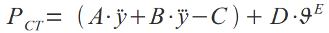
- The term in brackets is included only if > 0.
- If the measured lateral acceleration is in [m/s]
the coefficients A, B, C, D, E are as follows:
| Conditions |
A |
B |
C |
D |
E |
| In rest - standing |
28.542 |
20.693 |
11.1 |
0.185 |
2.283 |
| In rest - seated |
8.9704 |
9.6840 |
5.9 |
0.120 |
1.626 |
In the standard EN 12299 the acceleration is expressed in percent of gravitational acceleration,
why the original table is as follows:
| Conditions |
A |
B |
C |
D |
E |
| In rest - standing |
2.80 |
2.03 |
11.1 |
0.185 |
2.283 |
| In rest - seated |
0.88 |
0.95 |
5.9 |
0.120 |
1.626 |
- Text file example
HTML example
PDE Comfort on Discrete Events:
- Measure the lateral acceleration in the car-body
- Filter the acceleration in filter EN12299_PDE
- Calculate sliding average-, max- and min- value in a 2 [s] interval
- Calculate sliding peak value by subtracting the sliding max- and min- value
- Calculate PDE according to
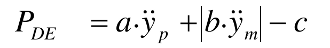
- If the measured lateral acceleration is in [m/s]
the coefficients a, b, c are as follows:
| Conditions |
a |
b |
c |
| In rest - standing |
16.616 |
27.013 |
37.0 |
| In rest - seated |
8.4608 |
13.048 |
21.7 |
In the standard EN 12299 the acceleration is expressed in percent of gravitational acceleration,
why the original table is as follows:
| Conditions |
a |
b |
c |
| In rest - standing |
1.63 |
2.65 |
37.0 |
| In rest - seated |
0.83 |
1.28 |
21.7 |
- Text file example
HTML example
Proposed scale in comfort units for NMV, NVA, NVD is as follows:
        N < 1           Very comfortable
    1 ≤ N < 2           Comfortable
    2 ≤ N < 4           Medium
    4 ≤ N < 5           Uncomfortable
    5 ≤ N               Very uncomfortable
Calculation of motion sickness value according to ISO 2631/3-1985
and ISO 2631-1:1997.
An evaluation has been carried out by ISO 2631/3 to study people's tendency
towards motion sickness.
It is stated in the norms that there are many factors in addition to motion,
that cause motion sickness among passengers.
It has, been difficult to formulate a good criterion, for other factors than vertical motion,
therefore only vertical motions is covered in the norm.
The acceleration has been measured at a point as far from the center of the car-body as possible,
in order to acquire the greatest possible vertical motion.
In the formulation of the norm,
only one frequency at a time has been studied in order to determine the requirement.
In case of an excitation comprising of several frequencies,
a broad-band analysis must be made where the entire
frequency register is computed, and a total RMS-value is calculated
according to Method 1).
The calculation of motion sickness according to ISO 2631/3-1985 is carried out by first
filtering the acceleration variable,
and then calculating the RMS value of the variable.
The RMS value equals the motion sickness value.
  Illustration of the vertical motion sickness filter ISOV_2631_3:

    ^
    |
    |                               The transfer function has the value
    |      ______                   "1" in interval  0.1-0.315 (Hz).
    |      |    |\
    |      |    | \
    |      |    |  \
    |      |    |   \
    |      |    |    \
    |      |    |     |
    |      |    |     |
    |      |    |     |
     ---------------------------->
          0.1  0.315  0.63        (Hz)
The filter ISOV_2631_3 has no physical background.
No frequencies over 0.63 Hz are taken into consideration,
nor will any frequencies under 0.1 Hz be taken into consideration.
According to ISO 2631/3-1985, it has been difficult to prove that frequencies
outside 0.1-0.63 Hz give rise to motion sickness.
In the ISO-analysis, the third octave band is from 0.1 to 0.63 Hz in filter ISOV_2631_3.
However, as every octave has a third octave width, this
will mean that the frequency range will be extended from 0.089 to 0.708.
In order to be able to calculate the risk of motion sickness according to ISO
2631/3, an example is given:
  Create_scalar new  Xeval_start= 120
  Create_scalar new  Xeval_stop = 2120
#
  Transt car_1b1.az           fname= car_1b1.az.ISO_MS85  type= ISOV_2631_3
  Transt car_1.m.az           fname= car_1.m.az.ISO_MS85  type= ISOV_2631_3
  Transt car_1b2.az           fname= car_1b2.az.ISO_MS85  type= ISOV_2631_3
  Stat   car_1b1.az.ISO_MS85  tname= lsb_11.pn   tstart= Xeval_start  tstop= Xeval_stop
  Stat   car_1.m.az.ISO_MS85  tname= lsc_1.pn    tstart= Xeval_start  tstop= Xeval_stop
  Stat   car_1b2.az.ISO_MS85  tname= lsb_12.pn   tstart= Xeval_start  tstop= Xeval_stop
In order to be able to calculate the risk of motion sickness according to ISO
2631-1:1997, an example is given:
  Create_scalar new  Xeval_start= 120
  Create_scalar new  Xeval_stop = 2120
#
  Transt car_1b1.az           fname= car_1b1.az.ISO_MS97  type= ISO2631_97WF
  Transt car_1.m.az           fname= car_1.m.az.ISO_MS97  type= ISO2631_97WF
  Transt car_1b2.az           fname= car_1b2.az.ISO_MS97  type= ISO2631_97WF
  Stat   car_1b1.az.ISO_MS97  tname= lsb_11.pn   tstart= Xeval_start  tstop= Xeval_stop
  Stat   car_1.m.az.ISO_MS97  tname= lsc_1.pn    tstart= Xeval_start  tstop= Xeval_stop
  Stat   car_1b2.az.ISO_MS97  tname= lsb_12.pn   tstart= Xeval_start  tstop= Xeval_stop
Output from the statistical calculation will be printed on the file \$ident.resu.
Example:.
 STATISTICS     for    car_1b1.az.    car_1.m.az.    car_1b2.az.
 ----------            ISO_MS85       ISO_MS85       ISO_MS85
 common exponent:       *E -3          *E -3          *E -3
   MAX    VALUE         39.316         37.327         44.755
   MIN    VALUE        -36.759        -34.646        -44.080
   RMS    VALUE         16.246         15.682         18.972  <- motion sickness value
   RMQ    VALUE         20.660         19.920         24.187
 AVERAGE  VALUE           .241           .230           .209
 MEDIAN                   .119           .370           .975
 STANDARD DEVIATION     16.245         15.680         18.971

 XVAR  WHEN MAX        924.000        649.333        646.667
 XVAR  WHEN MIN       1204.000       1476.000       1474.222
If only a part of the variable is used in the evaluation of the comfort
factor, the selection shall be made in the STAT command and not in the TRANS
command, as the TRANS command fill out the result with zeros in order to make Fname
to the same length as the input vector Iname.
Calculation of vertical motion sickness according to ISO 8041
ISO 8041 "Human response to vibration - Measuring instrumentation"
shows how a physical filter with poles and zeros can be designed
which is adapted to ISO 2631/3. The filter includes two fundamental parts,
a band pass filter and a frequency weighting filter.
The band pass filter is designed as follows:
 Hb(s) =             s2               ·          omega22
         (s2 + s·omega1/Q1 + omega12) · (s2 + s·omega2/Q1 + omega22)


 where omega1 = 0.49909   [rad/s]
       omega2 = 4.99090   [rad/s]
       Q1     = 0.7071067 [1]
The frequency weighting filter is designed as follows:
  Hms(s) =         1 + 0.105 · s
            (0.472·s)2 + 0.581·s + 1
In order to be able to calculate the motion sickness factor according to ISO
8041, an example is given:
Example:
  Create_scalar new  Xeval_start= 120
  Create_scalar new  Xeval_stop = 2120
#
  Transt car_1b1.az           fname= car_1b1.az.ISO_MS41  type= ISO8041V_MS
  Transt car_1.m.az           fname= car_1.m.az.ISO_MS41  type= ISO8041V_MS
  Transt car_1b2.az           fname= car_1b2.az.ISO_MS41  type= ISO8041V_MS
  Stat   car_1b1.az.ISO_MS41  tname= lsb_11.pn   tstart= Xeval_start  tstop= Xeval_stop
  Stat   car_1.m.az.ISO_MS41  tname= lsc_1.pn    tstart= Xeval_start  tstop= Xeval_stop
  Stat   car_1b2.az.ISO_MS41  tname= lsb_12.pn   tstart= Xeval_start  tstop= Xeval_stop
Output from the statistical calculation will be printed on file \$ident.resu.
Example:
 STATISTICS     for    car_1b1.az.    car_1.m.az.    car_1b2.az.
 ----------            ISO_MS41       ISO_MS41       ISO_MS41
 common exponent:       *E -3          *E -3          *E -3
   MAX    VALUE         41.254         37.554         50.971
   MIN    VALUE        -42.739        -34.946        -52.018
   RMS    VALUE         15.417         14.681         18.363  <- motion sickness value
   RMQ    VALUE         19.927         18.962         24.291
 AVERAGE  VALUE           .037           .028           .051
 MEDIAN                   .781           .876          1.591
 STANDARD DEVIATION     15.417         14.681         18.363

 XVAR  WHEN MAX        687.556        686.667        685.778
 XVAR  WHEN MIN        299.111        298.222        299.111
If only a part of the variable is used in the evaluation of the comfort
factor, the selection shall be made in the STAT command and not in the TRANS
command, as the TRANS command fill out the result with zeros in order to make Fname
to the same length as the input vector Iname.
Calculation of the motion sickness factor according to BS 6841:1987.
BS 6841:1987 is very similar to ISO 2631/3. The main difference is that a physical
filter has been adapted to the ideal curvature in ISO 2631/3. The filter in
BS 6841:1987 comprises a band pass filter in series with a filter which is called
frequency weight filter.
The band pass filter is designed as follows:
 Hb(s) =             s2               ·          omega22
         (s2 + s·omega1/Q1 + omega12) · (s2 + s·omega2/Q1 + omega22)


 where: omega1 = 0.5026548 [rad/s]
        omega2 = 3.9584067 [rad/s]
        Q1     = 0.71      [1]
The frequency weighting filter is designed as follows:
  Hw(s) = K * H4 * H5 * H6

  where:

                     omega42
  H4(s) = ----------------------------------
           (s2 + s*omega4/Q2 + omega42)


           (s2 + s*omega5/Q3 + omega52)
  H5(s) = ----------------------------------
                     omega52


                     omega62
  H6(s) = ----------------------------------
           (s2 + s*omega6/Q4 + omega62)


  K      = 0.4       [1]
  omega4 = 1.5707963 [rad/s]
  omega5 = 0.3926990 [rad/s]
  omega6 = 0.6283185 [rad/s]
  Q2     = 0.86      [1]
  Q3     = 0.80      [1]
  Q4     = 0.80      [1]
In order to calculate the motion sickness factor according to BS 6841:1987,
an example is given below:
  Create_scalar new  Xeval_start= 120
  Create_scalar new  Xeval_stop = 2120
#
  Transt car_1b1.az        fname= car_1b1.az.BS_WF     type= BS_WF
  Transt car_1.m.az        fname= car_1.m.az.BS_WF     type= BS_WF
  Transt car_1b2.az        fname= car_1b2.az.BS_WF     type= BS_WF
  Stat   car_1b1.az.BS_WF  tname= lsb_11.pn   tstart= Xeval_start  tstop= Xeval_stop
  Stat   car_1.m.az.BS_WF  tname= lsc_1.pn    tstart= Xeval_start  tstop= Xeval_stop
  Stat   car_1b2.az.BS_WF  tname= lsb_12.pn   tstart= Xeval_start  tstop= Xeval_stop
Output from the statistical calculation will be printed on file \$ident.resu.
Example:
 STATISTICS     for    car_1b1.az.BS car_1.m.az.BS car_1b2.az.BS
 ----------            _WF          _WF          _WF
 common exponent:       *E -3        *E -3        *E -3
   MAX    VALUE         20.087       18.801       24.729
   MIN    VALUE        -24.954      -22.399      -29.222
   RMS    VALUE          8.797        8.366        9.772  <- motion sickness value
   RMQ    VALUE         11.289       10.788       12.780
 AVERAGE  VALUE          -.013        -.008        -.024
 MEDIAN                   .003         .066         .502
 STANDARD DEVIATION      8.797        8.366        9.772

 XVAR  WHEN MAX        696.444      696.444      694.667
 XVAR  WHEN MIN        306.222      308.889      306.222
If only a part of the variable is used in the evaluation of the comfort
factor, the selection shall be made in the STAT command and not in the TRANST
command, as the TRANST command fill out the result with zeros in order to make Fname
to the same length as the input vector Iname.
5.3) Designing higher order filters.
In command FILT exists only first and second order, low and high pass filters.
If a filter of higher order is required it can created by making several
filtering in series.
5.3.1) Butterworth-filter
The Butterworth filter is a type of filter where the poles are equidistantly
placed in a half circle in the complex factor domain. The half circle only
exists for negative sigma values.
In a Butterworth filter all sub filters shall have the same cut-off frequency,
only the damping zeta shall be different according to the table below.
Filter's                                                     Approximate
Order    Filter    Filter type    Relative damping         relative damping

   2        1        lpass2_0       sin (π/4)                0.7071

   3        1        lpass1_0
            2        lpass2_0       sin (π/6)                0.5000

   4        1        lpass2_0       sin (π/8)                0.3827
            2        lpass2_0       sin (3*π/8)              0.9239

   5        1        lpass1_0
            2        lpass2_0       sin (π/10)               0.3090
            3        lpass2_0       sin (3*π/10)             0.8090

   6        1        lpass2_0       sin (π/12)               0.2588
            2        lpass2_0       sin (3*π/12)             0.7071
            3        lpass2_0       sin (5*π/12)             0.9659

   7        1        lpass1_0
            2        lpass2_0       sin (π/14)               0.2225
            3        lpass2_0       sin (3*π/14)             0.6235
            4        lpass2_0       sin (5*π/14)             0.9010

   8        1        lpass2_0       sin (π/16)               0.1951
            2        lpass2_0       sin (3*π/16)             0.5556
            3        lpass2_0       sin (5*π/16)             0.8315
            4        lpass2_0       sin (7*π/16)             0.9808

   9        1        lpass1_0
            2        lpass2_0       sin (π/18)               0.1736
            3        lpass2_0       sin (3*π/18)             0.5000
            4        lpass2_0       sin (5*π/18)             0.7660
            5        lpass2_0       sin (7*π/18)             0.9397

  10        1        lpass2_0       sin (π/20)               0.1564
            2        lpass2_0       sin (3*π/20)             0.4540
            3        lpass2_0       sin (5*π/20)             0.7071
            4        lpass2_0       sin (7*π/20)             0.8910
            5        lpass2_0       sin (9*π/20)             0.9877
Input data commands which controls plotting
In plotting MPLOT reads input data at different levels.
The levels are:
| MAIN | The highest level in program MPLOT.
Input data reading in MPLOT starts at this level |
| PAGE | The level that starts the definition of a new page. |
| DIAGRAM | The level that starts the definition of a new diagram in the page. |
CURVE
POINT
POINT_LINE
POINT3D | The lowest level consists of these four items.
This level controls the definition of a new curve or point in the diagram. |
Example:
Func,  Stat,        <---   In the beginning of the file, input are
Filt,...Etc.               read at level MAIN


Page 1             <---   Command to move input data reading to level PAGE


 Diagram 11        <---   Command to move input data reading to level DIAGRAM


  Curve            <---   Command to move input data reading to lowest level
                         Here you can define all data that is only valid
                         for this curve or point: yvar, xvar, line_type,
                         linetext, ...etc.
                         An EndCurve-command is not needed the curve- or point-
                         definition is finished by writing a new CURVE-, POINT-,
                         POINT_LINE-, POINT3D- or EndDiagram- command.


 EndDiagram        <---   Command to leave level DIAGRAM


EndPage            <---   Command to leave level PAGE and draw the page

                    <---   Back to level level MAIN again
When a new curve or point is to be created,
input data given under lowest level will have the highest priority,
and input data given under level MAIN will have the lowest priority.
Input data commands are not case sensitive, but variable names are.
Input data that valid at the lowest level
is also valid in the levels above level PAGE and level MAIN.
Therefore starts the input data descriptions at the lowest level:
Input data at the lowest input data level
The lowest input data level consists of the following levels:
| CURVE | Defines a curve to be plotted in actual diagram, the name of the curve is defined in command YVAR. |
| POINT | Defines a symbol to be plotted in actual diagram, the position of the symbol is defined in command YVAR and XVAR. |
| POINT_LINE | Defines a curve connecting the symbols defined by command POINT. |
| POINT3D | Defines a three-dimensional symbol to be plotted in actual diagram, the position of the symbol is defined in command ZVAR, YVAR and XVAR. |
Reference Manuals
MPLOT Main Menu
Level DIAGRAM
Input data valid at level CURVE
The CURVE command initializes the definition of a curve.
The Y-variable of the curve is defined in command YVAR.
The default X-variable of YVAR can be redefined by command XVAR.
The default ident can be redefined by command VAR_ID.
Command CURVE creates the text "Line" written to the left of the Y-axis.
The text can be supressed with command WRITE_ID.
| LINE_TYPE | = | Sets the type of line to be used. |
| LINETEXT | = | Explanatory text for the actual LINE_TYPE. |
| ROT_YTEXT | = | Rotation of the text to the left of the Y-axis. |
| VAR_ID | = | Sets the ident from which the variable shall be read from. |
| WRITE_YNAME | = | Controls the printing of YNAME. |
| WRITE_YTEXT | = | Controls the printing of all text to the left of the Y-axle. |
| XVAR | = | Select variable for the X-axle. |
| YNAME | = | Sets variable-name to be plotted at the Y-axis. |
| YVAR | = | Select variable for the Y-axle. |
| YVAR_EXPL | = | Explanation of YVAR. |
Reference Manuals
MPLOT Main Menu
Level DIAGRAM
Input data valid at level POINT
The POINT command indicates plotting of a point.
The Y-value of the point is defined in YVAR or YVALUE,
the X-value of the point is defined in XVAR or XVALUE.
Command POINT creates the text "Point" written to the left of the Y-axis.
The text can be supressed with command WRITE_ID.
| DOT_TYPE | = | Sets the type of symbols to be used |
| ROT_YTEXT | = | Rotation of the text to the left of the Y-axis. |
| VAR_ID | = | Sets the ident from which the variables shall be read. |
| WRITE_YNAME | = | Controls the printing of YNAME. |
| WRITE_YTEXT | = | Controls the printing of all text to the left of the Y-axle. |
| XVALUE | = | Manual input of the X-value for the point. |
| XVAR | = | Selects the scalar to be used as X-value of the point. |
| YNAME | = | Sets variable-name to be plotted at the Y-axis. |
| YVALUE | = | Manual input of Y-value to the point. |
| YVAR | = | Selects the scalar to be used as Y-value of the point. |
| YVAR_EXPL | = | Explanation of YVAR. |
Reference Manuals
MPLOT Main Menu
Level DIAGRAM
Input data valid at level POINT_LINE
The POINT_LINE command initializes the definition of a line which connects symbols
earlier defined in command POINT.
Command POINT_LINE creates the text "Pline" written to the left of the Y-axis.
The text can be supressed with command WRITE_ID.
Reference Manuals
MPLOT Main Menu
Level DIAGRAM
Input data valid at level POINT3D
The POINT3D command indicates plotting of a three-dimensional point.
The X-, Y- and Z-value of the point is defined in command XVAR, YVAR and ZVAR respectively.
The X-, Y- and Z-value of the point can also be given manually in command
XVALUE, YVALUE and
ZVALUE respectively.
Command POINT3D creates the text "Point" written to the left of the Y-axis.
The text can be supressed with command WRITE_ID.
| DOT_TYPE | = | Sets the type of symbols to be used |
| DRAW_ISOLINES | = | Drawing of contour lines. |
| ROT_YTEXT | = | Rotation of the text to the left of the Y-axis. |
| VAR_ID | = | Sets the ident from which the variables shall be read. |
| WRITE_YNAME | = | Controls the printing of YNAME. |
| XVALUE | = | Manual input of the X-value for the point. |
| XVAR | = | Selects the scalar to be used as X-value of the point. |
| YNAME | = | Sets variable-name to be plotted at the Y-axis. |
| YVALUE | = | Manual input of Y-value to the point. |
| YVAR | = | Selects the scalar to be used as Y-value of the point. |
| YVAR_EXPL | = | Explanation of YVAR. |
| ZVALUE | = | Manual input of the Z-value to point. |
| ZVAR | = | Select variable for the Z-axle. |
Reference Manuals
MPLOT Main Menu
Level DIAGRAM
Input data valid at level DIAGRAM
The DIAGRAM command initializes the definition of a local diagram.
Under level DIAGRAM all commands described under the lowest level
are available, plus the following commands:
| CALC_DATE | = | Date of calculation. |
| DIAG_HEIGHT | = | Defines the height of the diagram. |
| DIAG_WIDTH | = | Defines the width of the diagram. |
| HEAD | = | Set a diagram header line. |
| LIMIT_LINE | = | Define limit lines. |
| LIMIT_LINE_EXPL | = | Explanatory text for limit lines. |
| LXCM | = | Length of X-axis. |
| LYCM | = | Length of Y-axis. |
| ROT_YTEXT | = | Rotation of the text to the left of the Y-axis. |
| WRITE_CALC_DATE | = | Controls the printing of CALC_DATE. |
| WRITE_HEAD | = | Controls the printing of header lines. |
| WRITE_XNAME | = | Controls the printing of XNAME. |
| X_LEFT | = | The value of the X-axis on the left end. |
| X_MID | = | The value of the X-axis at the midpoint. |
| X_RIGHT | = | The value of the X-axis on the right end. |
| XAX_YVAL | = | Controls the location of the X-axis in the diagram. |
| XAXIS | = | Controls the plotting of the X-axis. |
| XCM/DEC | = | Logarithmic scaling factor in X-direction. |
| XGRID1 | = | Number of cm to the first grid line. |
| XGRIDINT | = | Number of cm between every vertical line in the grid. |
| XINT/CM | = | Scaling factor in X-direction. |
| XNAME | = | Sets the name to be plotted at the X-axis. |
| XVAR | = | Variable in X-direction. |
| XVAR_EXPL | = | Explanatory text for XVAR. |
| Y_BOT | = | The value of the Y-axis at the bottom end. |
| Y_MID | = | The value of the Y-axis at the midpoint. |
| Y_TOP | = | The value of the Y-axis at the top end. |
| YAXIS | = | Controls the plotting of the Y-axis. |
| YAX_XVAL | = | Controls the location of the Y-axis in the diagram. |
| YCM/DEC | = | Logarithmic scaling factor in the Y-direction. |
| YGRID1 | = | Number of cm to the first grid line. |
| YGRIDINT | = | Number of cm between every horizontal line in the grid. |
| YINT/CM | = | Scaling in the Y-direction. |
Commands to leave level DIAGRAM:
Reference Manuals
MPLOT Main Menu
Level DIAGRAM
Input data valid at level PAGE
The PAGE command initializes the definition of a new page.
Under level PAGE all commands described under level DIAGRAM
are available, plus the following commands:
Commands to leave level PAGE:
Reference Manuals
MPLOT Main Menu
Level PAGE
Input data valid at level MAIN
The ENDPAGE command finalizes current page definition and input data reading continues at level MAIN.
Under level MAIN all commands described under level PAGE are available,
plus the following commands:
| ILASER | = | Indicator for writing the graphs to a printer. |
| INKFIL | = | Controls the writing of a debug logging file. |
| ISCREN | = | Indicator for plotting on the screen. |
| MPLOT_DATE | = | Current date, shown in the upper right-hand corner of the title. |
| MPLOT_ID | = | Ident for this plotting activity. |
| PAPER_FORMAT | = | Defines the size of the paper to be used. |
| POSTFI | = | Graphic output data file. |
| VAR_DIR | = | Directory where the calculation results are stored. |
Commands to leave level MAIN:
| PAGE | = | Initializes the definition of a new page. |
Reference Manuals
MPLOT Main Menu
Level MAIN
All plotting commands in alphabetical order
Reference Manuals
MPLOT Main Menu
Alphabetical list
CALC_DATE
Date of calculation, shown under each diagram.
See also: LOC_CALC_DATE, SIZE_CALC_DATE, WRITE_CALC_DATE
Declared= Character*80 Default= The date read from the MPdat-file
CURVE
The CURVE command initializes the definition of a new curve
and moves the input data reading to level CURVE.
DIAG_HEIGHT
Defines the hight of the diagram.
| Declared | = | Real*4 |
| Default | = | The height of PAPER_FORMAT minus margins divided by NROWS. |
DIAG_WIDTH
Defines the width of the diagram.
DIAGRAM diag_no
Read the diagram number and move input data reading to level DIAGRAM.
| diag_no |
= |
Diagram number.
The page is divided into a number of smaller drawing areas, defined by diag_no.
The small drawing areas are numbered, in rows and columns similar to the components in a
matrix, i.e. the first row is numbered 11,12, 13, ... etc.
The next row is numbered 21,22,23,...etc.
Max. number of columns are limited to 9.
Number of rows can be bigger then 10,
but total number of drawing areas must be less than 160.
Declared= Integer*4
|
DOT_TYPE
Defines the shape of the dots used when plotting scalars.
| Declared | = | Integer*4 |
| Default | = | 'AUTO' i.e. the first point is plotted with DOT_TYPE 2, point 2 with DOT_TYPE 3 etc. |
DRAW_ISOLINES = DIAG_NO, METHOD, LEVELS
Drawing of isolines, for points which are defined with the command
DIAGPT3D. The command demands that the points lie in a grid, and are
numbered with point number 1 at the top left-hand corner, and point
2 to the right of point 1 etc. downwards in rows until the last point
is located at the bottom to the right. This also implies that every
line is equally long, and every column equally high. Long and high
refer to the number of points in the lines and columns, however it
is not required that the points are located at a equidistant spacing
from each other.
| DIAG_NO | = | Defines the diagram number, line and column- number.
Declared= Integer*4
Default = 11 |
| METHOD | = | Sets the method of drawing the isolines.
Following values are valid for METHOD:
'NO'= cancels the drawing of isolines.
'LIN'= linear interpolation between the points.
Declared= Character*20
Default = 'NO' |
| LEVELS | = | Numerical values of the hight of the isolines to be drawn.
If LEVELS is set to a negative value,
LEVELS will control the number of lines to be drawn in the diagram.
Declared= Real*4
Default = 0 |
ENDDIAGRAM
The ENDDIAGRAM command ends current diagram definition and returns the input data reading to
level PAGE.
ENDPAGE
The ENDPAGE command ends the current page definition, and writes the output on screen and/or file.
After command ENDPAGE further input data will be read at level MAIN.
EXEC
Terminates the ongoing command.
Certain commands are not executed until a new main-command has been read.
This is due to the fact that the amount of input data is not known from the outset.
After program MPLOT have read command EXEC, further input data reading will continue
at level MAIN
FRAME
Controls the drawing of the frame around the diagrams.
Following values are valid:
| GLOBAL | = | draws a large frame around the entire page. |
| LOCAL | = | draws a frame around each diagram. |
| GLOBAL_LOCAL | = | draws both global and local frames. |
| NO | = | suppresses the drawing of frames. |
Declared= Character*12 Default= GLOBAL_LOCAL
HEAD= head_no, htext
Input of text header lines, written in the diagrams.
| head_no |
= |
Head line number to be read.
Valid values for head_no are between 1 and 10.
Declared= Integer*4 |
| htext |
= |
The text of the header line.
Declared= Character*80(10) |
In the header lines the user has the possibility to retrieve values of scalars.
In order to retrieve a value from a scalar, the user shall write the name of the
scalar with a \$-sign in the beginning of the name of the scalar.
The following example retrieves the values the ride comfort indexes
in current ident:
 head1= 'Wz.m=$car_1.m.ayWZ   RMS.m=$car_1.m.ay.ERRMS'
 head2= 'Wzb1=$car_1b1.ayWZ   RMSb1=$car_1b1.ay.ERRMS'
 head3= 'Wzb2=$car_1b2.ayWZ   RMSb2=$car_1b2.ay.ERRMS'
The following example retrieves the values the ride comfort indexes
in other idents:
 head1= 'Wz.m=$car_1.m.ayWZ(ident_001)   RMS.m=$car_1.m.ay.ERRMS(ident_001)'
 head2= 'Wz.m=$car_1.m.ayWZ(ident_002)   RMS.m=$car_1.m.ay.ERRMS(ident_002)'
 head3= 'Wz.m=$car_1.m.ayWZ(ident_003)   RMS.m=$car_1.m.ay.ERRMS(ident_003)'
If the user wishes the heading text to be retrieved from the MPdat-file,
the following sub directives can be given in command HEAD:
| IDENT | = | Ident string from where the headers will be retrieved.
Declared= Character*100 |
| HEAD | = | Number of the head line which will be retrieved.
Declared= Integer*4 |
Example:
 head1= IDENT= ident_001    HEAD= 3
 head2= IDENT= ident_001    HEAD= 2
 head3= IDENT= ident_001    HEAD= 1
See also:
LOC_HEAD,
SIZE_HEAD,
WRITE_HEAD.
ILASER
Format for graphic output.
Valid values for ILASER are:
intro_common_commands.html#jILASER
Declared= Integer*4 Default= 6
INKFIL
Controls the writing of a debug logging file.
Command INKFIL can be switched on and off several times during the plotting activity.
INKFIL can be given the following values:
0 => No printing.
3 => Print of log file to the file code 03.
6 => Print of log file to the file code 06 i.e. standard output.
Declared= Integer*4 Default= 0
ISCREN
Declared= Integer*4 Default= 0
LIMIT_LINE = LINE_NO, +-`YLIM1, +-`XLIM1, +-`YLIM2, +-`XLIM2
Creation of limit lines in the diagram.
| LINE_NO | = |
The number of the limit line.
Up to four limit lines can be defined.
Declared= Integer*4
Default = 'NONE' |
| YLIM1 | = |
The limit of the left-hand side of the diagram.
If only YLIM1 is specified, the limit will assume to be
horizontal and will extend over the entire diagram.
Declared= Real*4
Default = 'NONE' |
| XLIM1 | = |
X-coordinate for the start of the limit line.
Declared= Real*4
Default = 'LEFT' i.e. at the beginning of the X-axis. |
| YLIM2 | = |
The right-hand side limit of the diagram.
Declared= Real*4
Default = 'NONE' |
| XLIM2 | = |
X-coordinate for the right end of the limit line.
If XLIM2 is not specified, the program will assume that the
limit line will extend across the entire diagram.
Declared= Real*4
Default = 'RIGHT' i.e. the end of the X-axis. |
LIMIT_LINE_EXPL = LINE_NO, EXPL_TEXT
Explanatory text for LIMIT_LINE.
| LINE_NO | = | The number of the limit line to be explained.
Declared= Integer*4
Default = 'NONE' |
| EXPL_TEXT | = | Text to be written above the diagram, will be written if it is non-blank.
Declared= Character*80
Default = Blank |
See also: LOC_LIMIT_EXPL, SIZE_LIMIT_EXPL
LINE_TYPE= LINE_TYPE, THICKNESS, LINE_DOTS
Command LINE_TYPE determines the type of line to be used when drawing curves.
LINE_TYPE controls the color and shape of the curves.
| LINE_TYPE | = |
Defines type of line to be drawn.
Following values are valid for LINE_TYPE:
| Declared | = | Integer*4 |
| Default | = | 'AUTO' i.e. the first line is plotted with line type 1, line 2 with line type 2 etc. |
|
| THICKNESS | = | Defines the width of the line to be drawn.
Following values are valid:
0= No line.
1= Thinnest possible line.
2= Slightly thicker line.
3= Thicker line etc.
Declared= Integer*4 Default= 1
|
| LINE_DOTS | = | Sets if symbols shall be drawn at all nodes along the curve.
Following values are valid:
0= No symbols are drawn.
1= A symbol is drawn at all nodes.
Type of symbol to be drawn at the nodes is defined in DOT_TYPE.
Declared= Integer*4 Default= 0
|
LINETEXT
Explanatory text for the actual LINE_TYPE.
The text is written if it is non-blank.
See also: LOC_LINETEXT, SIZE_LINETEXT
Declared= Character*80 Default= " " (Blank)
LOC_CALC_DATE
Controls the location of CALC_DATE.
| Declared | = | Real*4(2) Units= [cm] |
| Default | = | AUTO i.e. In the lower right-hand corner. |
LOC_DIAG_LL
Location of the lower left corner of the DIAGRAM.
| Declared | = | Real*4(2) Units= [cm] |
| Default | = | AUTO i.e. the diagrams are close-packed |
LOC_FRAME_LL
Location of the lower left corner of the drawing area,
in relation to the lower left corner of the local DIAGRAM.
| Declared | = | Real*4(2) Units= [cm] |
| Default | = | AUTO i.e. the drawing area is placed in the middle of the DIAGRAM |
LOC_HEAD= head_no, x-value, y-value
Controls the position of the HEAD-lines.
| head_no | = | Number of the HEAD-line.
Valid values for head_no are between 1 and 10.
Declared= Integer*4 |
| x-value | = | The X-coordinate of the lower left corner.
Declared= Real*4 Units= [cm] |
| y-value | = | The Y-coordinate of the lower left corner.
Declared= Real*4 Units= [cm] |
LOC_LIMIT_EXPL
Sets the location of LIMIT_LINE_EXPL.
| Declared | = | Real*4(2) Units= [cm] |
| Default | = | AUTO i.e. above the diagram. |
LOC_LINETEXT
Controls the location of the text defined in command LINETEXT.
| Declared | = | Real*4(2) Units= [cm] |
| Default | = | Above the diagram originating from the left-hand side. |
LOC_MPLOT_DATE
Controls the location of MPLOT_DATE.
| Declared | = | Real*4(2) Units= [cm] |
| Default | = | AUTO i.e. at the top right-hand side of the page. |
LOC_MPLOT_ID
Controls the location of MPLOT_ID.
| Declared | = | Real*4(2) Units= [cm] |
| Default | = | AUTO i.e. at the upper right-hand side of the page |
LOC_PAGE_HEAD= head_no, x-value, y-value
Controls the position of PAGE_HEAD.
| head_no | = | Number of the PAGE_HEAD-line.
Valid values for head_no are between 1 and 10.
Declared= Integer*4 |
| x-value | = | The X-coordinate of the lower left corner.
Declared= Real*4 Units= [cm] |
| y-value | = | The Y-coordinate of the lower left corner.
Declared= Real*4 Units= [cm] |
LOC_PAGE_NO
Controls the location of the page number in X- and Y-coordinates.
| Declared | = | Real*4(2) Units= [cm] |
| Default | = | AUTO i.e. at the upper right-hand side of the page |
LOC_VAR_ID
Sets the location of VAR_ID.
| Declared | = | Real*4(2) Units= [cm] |
| Default | = | To the left of YNAME. |
LOC_XNAME
Sets the location of XNAME.
| Declared | = | Real*4(2) Units= [cm] |
| Default | = | AUTO i.e. under the X-axis to the right. |
LOC_XVAR_EXPL
Sets the location of XVAR_EXPL.
| Declared | = | Real*4(2) Units= [cm] |
| Default | = | AUTO i.e. to the right of XNAME. |
LOC_YNAME
Controls the location of YNAME.
| Declared | = | Real*4(2) Units= [cm] |
| Default | = | AUTO i.e. on the top left-hand side of the Y-axis. |
LOC_YVAR_EXPL
Controls the location of YVAR_EXPL.
| Declared | = | Real*4(2) Units= [cm] |
| Default | = | AUTO i.e. to the right of YVAR. |
LXCM
Sets the length of the X-axis.
| Declared | = | Real*4 Units= [cm] |
| Default | = | 'AUTO' i.e. Maximum length within DIAG_WIDTH |
LYCM
Sets the length of the Y-axis.
| Declared | = | Real*4 Units= [cm] |
| Default | = | 'AUTO' i.e. Maximum length within DIAG_HEIGHT |
MPLOT_DATE
Current date, shown in the upper right-hand corner of the title.
See also: LOC_MPLOT_DATE, SIZE_MPLOT_DATE, WRITE_MPLOT_DATE
Declared= Character*80 Default= Current date
MPLOT_ID
Ident for current plotting activity,
plotted in the upper right corner of the title.
Can be set in this command or given in Command Line Options.
See also: LOC_MPLOT_ID, SIZE_MPLOT_ID, WRITE_MPLOT_ID
Declared= Character*80 Default= "mplot_id"
NCOLS
Defines number of columns of local diagrams.
See also: NROWS
| Declared | = | Integer*4 |
| Default | = | 'AUTO' i.e. diag_no-(floor(diag_no/10))*10 where diag_no is defined in DIAGRAM. |
NOTE
Commentary line, the rest of the line is ignored.
Declared= Character*80 Default= Blank
NROWS
Defines number of rows of local diagrams.
See also: NCOLS
| Declared | = | Integer*4 |
| Default | = | 'AUTO' i.e. floor(diag_no/10) where diag_no is defined in DIAGRAM. |
OVERWRITE
States the area of which the curves may be plotted.
Following values are valid:
| GLOBAL | = | Allows curves to be plotted over the whole PAGE. |
| LOCAL | = | Allows curves to be plotted over the whole local DIAGRAM. |
| NO | = | Allows only curves to be plotted in the drawing area of the local DIAGRAM. |
Declared= Character*6 Default= 'NO'
PAGE page_no
Read page number and move input data reading to level PAGE.
Declared= Integer*4 Default= "Previous page number" + 1
PAGE_HEAD= head_no, htext
Text header lines, written above the diagrams.
| head_no | = | Head line number to be read.
Valid values for head_no are between 1 and 10.
Declared= Integer*4 |
| htext | = | The text of the header line.
Declared= Character*80(10) |
If the user wishes the header line to be read from a MPdat-file,
htext can be replaced by the sub-directives IDENT and HEAD:
| IDENT | = | Ident from where the head lines shall be read.
Declared= Character*80 |
| HEAD | = | Number of the head line to be read.
Declared= Integer*4 |
See also:
LOC_PAGE_HEAD,
SIZE_PAGE_HEAD,
WRITE_PAGE_HEAD.
PAPER_FORMAT
Defines the size of the paper to be used.
The orientation of the paper is controlled in command XAXIS_ALONG.
Following values are valid:
A0 => Selects paper A0.
A1 => Selects paper A1.
A2 => Selects paper A2.
A3 => Selects paper A3.
A4 => Selects paper A4.
Declared= Character*2 Default= 'A4'
POINT
The POINT command initializes the definition of a new symbol
and moves the input data reading to level POINT.
POINT_LINE method, p_id
The POINT_LINE command initializes the definition of a new curve
and moves the input data reading to POINT_LINE.
POINT_LINE plots a curve, fitted to the points given by command POINT.
| method | = | Controls the method of which the line will be drawn.
Following values are valid:
| POLYGON | = | polygon through the points. |
| LEASTSQ_LIN_LIN | = | linear regression in a lin-lin diagram. |
| LEASTSQ_LIN_LOG | = | linear regression in a lin-log diagram. |
| LEASTSQ_LOG_LIN | = | linear regression in a log-lin diagram. |
| LEASTSQ_LOG_LOG | = | linear regression in a log-log diagram. |
| SPLINE_LIN_LIN | = | cubic splines in a lin-lin diagram. |
| SPLINE_LIN_LOG | = | cubic splines in a lin-log diagram. |
| SPLINE_LOG_LIN | = | cubic splines in a log-lin diagram. |
| SPLINE_LOG_LOG | = | cubic splines in a log-log diagram. |
Declared= Character*20
Default = 'LEASTSQ_LIN_LIN' |
| p_id | = | List of the numbers of the points, which shall be taken into consideration when drawing the curve.
If P_ID = 'ALL', all points will be used when the drawing the curve.
Declared= Integer*4(1000) Default= 'ALL'
|
POINT3D
The POINT3D command initializes the definition of a three-dimensional point
and moves the input data reading to level POINT3D.
POSTFI
Sets the name of the graphic output data file.
See also: ILASER
Declared= Character*80 Default= "\$ident.ps"
QUIT, STOP or EXIT
End the execution of program MPLOT.
ROT_YTEXT
Controls the rotation in degrees of the text to the left of the Y-axis.
The scale to the left of the Y-axis can be rotated in a arbitrary angle.
The text strings WRITE_ID, VAR_ID, YNAME and YVAR_EXPL
are rotated 0. or 180. degrees.
The rotation is a right handed rotation.
Which means that setting ROT_YTEXT= -90 vill give a scale with upright numbers.
If ROT_YTEXT is set equal to -90 you may also want to make more space to the left of the Y-axis.
This can be made with the LOC_FRAME_LL-command.
Declared= Real*4 Default = 180. [deg]
SIZE_CALC_DATE
Controls the character size of CALC_DATE.
Declared= Real*4 Default = .175 [cm]
SIZE_HEAD
Controls the character size of HEAD.
Declared= Real*4 Default = .175 [cm]
SIZE_LIMIT_EXPL
Controls the character size of LIMIT_LINE_EXPL.
Declared= Real*4 Default = .175 [cm]
SIZE_LINETEXT
Controls the character size of LINETEXT.
Declared= Real*4 Default = .175 [cm]
SIZE_MPLOT_DATE
Controls the character size of MPLOT_DATE.
Declared= Real*4 Default = .2 [cm]
SIZE_MPLOT_ID
Controls the size of MPLOT_ID.
Declared= Real*4 Default= .2 [cm]
SIZE_PAGE_HEAD
Controls the size of PAGE_HEAD.
Declared= Real*4 Default= AUTO, max. .25 [cm]
SIZE_PAGE_NO
Controls the size of the page number.
Declared= Real*4 Default= .2 [cm]
SIZE_XNAME
Controls the size of XNAME.
Declared= Real*4 Default= .175 [cm]
SIZE_YNAME
Controls the size of YNAME.
Declared= Real*4 Default= .175 [cm]
VAR_DIR
Directory where the calculation results are stored.
Declared= Character*80 Default= "." i.e. current directory
VAR_ID
Sets the ident from which the variable shall be read.
Following
wildcards
are allowed:
| ? |
matches any single character in a filename |
| * |
matches any string of characters (including the empty string) in a filename |
| [ ] |
matches any single character from the set enclosed in the brackets |
See also: LOC_VAR_ID, WRITE_VAR_ID
WRITE_CALC_DATE
Controls the plotting of CALC_DATE.
Following values are valid:
'Y' or 'YES' indicates that the date will be plotted.
'N' or 'NO' indicates that the date will not be plotted.
Declared= Character*3 Default= 'N'
WRITE_HEAD= head_no, value
Controls the printing of HEAD-lines.
| head_no | = | Number of the HEAD-line to be printed or not.
Valid values for head_no are between 1 and 10.
Declared= Integer*4 |
| value | = | Sets if the HEAD-line shall be printed or not.
Valid values are 'Y' or 'N'.
Declared= Character*3(10) |
WRITE_ID
Gives information which command that has created the curve or point
| Level | Text to be written to the left of the Y-axis: |
| CURVE | "Line" |
| POINT | "Point" |
| POINT3D | "Point" |
| POINT | "Pline" |
'Y' or 'YES' indicates that the text will be printed.
'N' or 'NO' indicates that the tex will not be printed.
Declared= Character*3 Default = 'Y'
WRITE_MPLOT_DATE
Controls the printing of MPLOT_DATE.
'Y' or 'YES' states that the date will be printed
'N' or 'NO' states that the date will not be printed
Declared= Character*3 Default= 'Y'
WRITE_MPLOT_ID
Controls the plotting of current ident MPLOT_ID.
'Y' or 'YES' states that the plot ident will be plotted.
'N' or 'NO' states that the plot ident will not be plotted.
Declared= Character*3 Default= 'Y'
WRITE_PAGE_HEAD= head_no, value
Controls the printing of PAGE_HEAD-lines.
| head_no | = | Number of the PAGE_HEAD-line to be printed or not.
Valid values for head_no are between 1 and 10.
Declared= Integer*4 |
| value | = | Sets if the PAGE_HEAD-line shall be printed or not.
Valid values are 'Y' or 'N'.
Declared= Character*3(10) |
WRITE_PAGE_NO
Controls the plotting of page number.
'Y' or 'YES' indicates that the page number will be plotted.
'N' or 'NO' indicates that the page number will not be plotted.
Declared= Character*3 Default= 'Y'
WRITE_VAR_ID
Controls the plotting of VAR_ID.
Following values are valid:
'Y' or 'YES' indicates that the ident text will be printed.
'N' or 'NO' indicates that the ident text will not be printed.
Declared= Character*3 Default= 'Y'
WRITE_XNAME
Controls the plotting of XNAME.
Following values are valid:
'Y' or 'YES' indicates that the text will be printed.
'N' or 'NO' indicates that the text will not be printed.
Declared= Character*3 Default = 'Y'
WRITE_YNAME
Controls the plotting of YNAME.
Following values are valid:
'Y' or 'YES' indicates that the text will be printed.
'N' or 'NO' indicates that the text will not be printed.
Declared= Character*3 Default= 'Y'
WRITE_YTEXT
Controls the plotting of all text to the left of the Y-axis,
i.e. all of WRITE_ID,
WRITE_VAR_ID and
WRITE_YNAME.
Following values are valid:
'Y' or 'YES' indicates that all Y-text will be printed.
'N' or 'NO' indicates that no Y-text will not be printed.
Declared= Character*3 Default= 'Y'
X_LEFT
Sets the left-hand value of the X-axis.
This input data is equal to the commands X_MID and X_RIGHT,
the last given input data command will apply.
X_LEFT, X_MID and X_RIGHT shall all be set to 'AUTO' if automatic scaling is desired.
A special case occurs if both X_LEFT and X_RIGHT are defined but not XCM/DEC.
In that case XINT/CM will be set to (X_RIGHT-X_LEFT)/LXCM and the MARKINGS-distance
in the XAXIS-command will be set to a suitable value in order to give integer numbers
at the X-axis.
This special case do only occur if X_LEFT and X_RIGHT is given under level DIAGRAM,
and please set XGRIDINT equal to 'AUTO'.
See also: X_MID, X_RIGHT, XINT/CM,
Declared= If text: Character*4 else Real*4
Default = 'AUTO'
X_MID
Sets the value of the X-axis at the midpoint of the axis.
This input data is equal to the commands X_LEFT and X_RIGHT,
the last given input data command will apply.
X_LEFT, X_MID and X_RIGHT shall all be set to 'AUTO' if automatic scaling is desired.
See also: X_LEFT, X_RIGHT, XINT/CM,
Declared= If text: Character*4 else Real*4
Default = 'AUTO'
X_RIGHT
Sets the right-hand value of the X-axis.
This input data is equal to the commands X_MID and X_LEFT,
the last given input data command will apply.
X_LEFT, X_MID and X_RIGHT shall all be set to 'AUTO' if automatic scaling is desired.
A special case occurs if both X_LEFT and X_RIGHT are defined but not XCM/DEC.
In that case XINT/CM will be set to (X_RIGHT-X_LEFT)/LXCM and the MARKINGS-distance
in the XAXIS-command will be set to a suitable value in order to give integer numbers
at the X-axis.
This special case do only occur if X_LEFT and X_RIGHT is given under level DIAGRAM,
and please set XGRIDINT equal to 'AUTO'.
See also: X_MID, X_RIGHT, XINT/CM,
Declared= If text: Character*4 else Real*4
Default = 'AUTO'
XAX_YVAL
Controls the location of the X-axis in the diagram.
XAX_YVAL refers to the value where the X-axis will meet the Y-axis.
Instead of giving a Y-value, following character strings are understood:
| 'BOT' | = | The X-axis is placed at the bottom of the Y-axis. |
| 'MID' | = | The X-axis is placed at the midpoint of the Y-axis. |
| 'TOP' | = | The X-axis is placed at the top of the Y-axis. |
Declared= If text: Character*3 else Real*4 Units= [cm]
Default = 'BOT'
XAXIS = TYPE, MARKINGS, FIGURES
Controls the plotting of the X-axis.
| TYPE | = |
Sets the type of scale to be used.
Following values are valid:
'LIN' = linear scale.
'LOG' = logarithmic scale.
'OFF' = cancels the plotting of the X-axis.
Declared= Character*3
Default = 'LIN' |
| MARKINGS | = |
Sets the length in cm between the markings on the X-axis.
In use of the logarithmic scale, MARKINGS are used
as the minimum distance between the two consecutive markings.
MARKINGS = 0 cancels the print.
Declared= Real*4
Default = 1 [cm] |
| FIGURES | = |
Sets how often the axle markings will be marked with a figure.
Following values are valid for FIGURES:
1 = a figure on every axis marking.
2 = a figure on every second axis marking.
3 = a figure on every third axis marking,,, etc.
0 = cancels the print of figures.
Declared= Real*4
Default = 2 |
XAXIS_ALONG
Orientation of the X-axis.
Following values are valid:
| LONG_SIDE | gives a diagram in landscape format |
| SHORT_SIDE | gives a diagram in portrait format |
Declared= Character*12 Default= 'LONG_SIDE'
XCM/DEC
Sets the scale factor of the X-axle, if XAXIS has been set to 'LOG'.
XCM/DEC defines the number of cm per decade.
See also: X_LEFT, X_MID, X_RIGHT, XINT/CM
Declared= If text: Character*4 else Real*4
Default = 'AUTO' (i.e. a value from the following series: 1,2,5,10,20,...etc.)
XGRID1
Sets number of cm from the Y-axis to the first grid line.
See also: XGRIDINT
Declared= If text: Character*4 else Real*4
Default = 'AUTO' i.e. same distance as to the first axis marking.
XGRIDINT
Sets the number of cm between every vertical line of the grid.
The grid pattern is drawn with LINE_TYPE= 2.
See also: XGRID1
Declared= If text: Character*4 else Real*4
Default = 'AUTO' i.e. same distance as the axis markings.
XINT/CM
Sets the scale factor of the X-axle, if XAXIS has been set to 'LIN'.
XINT/CM defines the number of units per cm.
See also: X_LEFT, X_MID, X_RIGHT, XCM/DEC
Declared= If text: Character*4 else Real*4
Default = 'AUTO' (i.e. a value from the following series: 1,2,5,10,20,...etc.)
XNAME
Sets variable-name to be plotted at the X-axis.
See also: LOC_XNAME, SIZE_XNAME, WRITE_XNAME
Declared= Character*80
Default = Same name as XVAR.
XVALUE
Manually set the X-value of the point.
Declared= Real*4
Default = The value of XVAR
XVAR
Select variable for the X-axle.
The user can draw a X-variable from an another ident, by defining
the name of the ident inside parenthesis: XVAR= var_name(ident)
Different curves can have different X-variables,
but the text under the X-axle will be picked from XVAR(1).
Declared= Character*80(200)
Default = The default X-variable of YVAR.
XVAR_EXPL
Explanatory text of XVAR.
The text is printed if it is non-blank.
The text is printed with the same text size as XNAME.
See also: LOC_XVAR_EXPL
Declared= Character*80 Default= " "(Blank)
Y_BOT
The value of the Y-axis at the bottom of the axis.
This input data is equal to the commands Y_MID and Y_TOP,
the last given input data command will apply.
Y_BOT, Y_MID and Y_TOP shall all be set to 'AUTO' if automatic scaling is desired.
A special case occurs if both Y_BOT and Y_TOP are defined but not YINT/CM.
In that case YINT/CM will be set to (Y_BOT-Y_TOP)/LYCM and the MARKINGS-distance
in the YAXIS-command will be set to a suitable value in order to give integer numbers
at the Y-axis.
This special case do only occur if Y_BOT and Y_TOP is given under level DIAGRAM,
and please set YGRIDINT equal to 'AUTO'.
See also: Y_MID, Y_TOP, YINT/CM,
Declared= If text: Character*4 else Real*4
Default = 'AUTO'
Y_MID
The value of the Y-axis at the middle of the axis.
This input data is equal to the commands Y_BOT and Y_TOP,
the last given input data command will apply.
Y_BOT, Y_MID and Y_TOP shall all be set to 'AUTO' if automatic scaling is desired.
See also: Y_BOT, Y_TOP, YINT/CM,
Declared= If text: Character*4 else Real*4
Default = 'AUTO'
Y_TOP
The value of the Y-axis at the top of the axis.
This input data is equal to the commands Y_MID and Y_BOT,
the last given input data command will apply.
Y_BOT, Y_MID and Y_TOP shall all be set to 'AUTO' if automatic scaling is desired.
A special case occurs if both Y_BOT and Y_TOP are defined but not YINT/CM.
In that case YINT/CM will be set to (Y_BOT-Y_TOP)/LYCM and the MARKINGS-distance
in the YAXIS-command will be set to a suitable value in order to give integer numbers
at the Y-axis.
This special case do only occur if Y_BOT and Y_TOP is given under level DIAGRAM,
and please set YGRIDINT equal to 'AUTO'.
Declared= If text: Character*4 else Real*4
Default = 'AUTO'
YAX_XVAL
Controls the location of the Y-axis in the diagram.
YAX_XVAL refers to the value where the Y-axis will meet the X-axis.
Instead of giving a X-value, following character strings are understood:
| 'LEFT' | = | The Y-axis is placed at the left of the X-axis. |
| 'MID' | = | The Y-axis is placed at the midpoint of the X-axis. |
| 'RIGHT' | = | The Y-axis is placed at the right of the X-axis. |
Declared= If text: Character*5 else Real*4 Units= [cm]
Default = 'LEFT'
YAXIS = TYPE, MARKINGS, FIGURES
Controls the plotting of the Y-axis.
| TYPE | = |
Sets the type of scale to be used.
Following values are valid:
'LIN' = linear scale.
'LOG' = logarithmic scale.
'OFF' = cancels the plotting of the Y-axis.
Declared= Character*3
Default = 'LIN' |
| MARKINGS | = |
Sets the length in cm between the markings on the Y-axis.
In use of the logarithmic scale, MARKINGS are used
as the minimum distance between the two consecutive markings.
MARKINGS = 0 cancels the print.
Declared= Real*4
Default = 1 [cm] |
| FIGURES | = |
Sets how often the axle markings will be marked with a figure.
Following values are valid for FIGURES:
1 = a figure on every axis marking.
2 = a figure on every second axis marking.
3 = a figure on every third axis marking,,, etc.
0 = cancels the print of figures.
Declared= Real*4
Default = 1 |
YCM/DEC
Sets the scale factor of the Y-axle, if YAXIS has been set to 'LOG'.
YCM/DEC defines the number of cm per decade.
See also: Y_TOP, Y_MID, Y_BOT, YINT/CM
Declared= If text: Character*4 else Real*4
Default = 'AUTO' (i.e. a value from the following series: 1,2,5,10,20,...etc.)
YGRID1
Sets the number of cm from the x-axis to the first grid line.
See also: YGRIDINT
Declared= If text: Character*4 else Real*4
Default = 'AUTO' i.e. same distance as to the first axis marking.
YGRIDINT
Sets the number of cm between every horizontal line in the grid.
The grid pattern is drawn with LINE_TYPE= 2.
See also: YGRID1
Declared= If text: Character*4 else Real*4
Default = 'AUTO' i.e. same distance as the axis markings.
YINT/CM
Sets the scale factor of the Y-axle, if YAXIS has been set to 'LIN'.
YINT/CM defines the number of units per cm.
See also: Y_BOT, Y_MID, Y_TOP, YCM/DEC
Declared= If text: Character*4 else Real*4
Default = 'AUTO' (i.e. a value from the following series: 1,2,5,10,20,...etc.)
YNAME
Sets variable-name to be plotted at the Y-axis.
See also: LOC_YNAME, SIZE_YNAME, WRITE_YNAME
Declared= Character*80
Default = Same name as YVAR.
YVALUE
Manually set the Y-value of the point.
Declared= Real*4
Default = The value of YVAR
YVAR
Select variable to draw in the diagram.
The user can draw an Y-variable from an another ident, by defining
the name of the ident inside parenthesis: YVAR= var_name(ident)
The variable for the X-axle is defined in XVAR.
If XVAR is undefined,
the default X-variable of YVAR will apply.
In order to draw the curve upside-down, the variable can be preceded by a "-" sign.
However in this case the auto-scale will not work.
The user must manually set the scale factor in command YINT/CM.
Declared= Character*80(200)
Default = 'NONE' i.e. no Y-variable.
YVAR_EXPL
Explanatory text of YVAR.
The text is printed if it is non-blank.
The text is printed with the same text size as YNAME.
See also: LOC_YVAR_EXPL
Declared= Character*80 Default= " "(Blank)
ZVALUE
Manually set the Z-value of the point.
Declared= Real*4
Default = The value of ZVAR
ZVAR
Selects the scalar to be used as Z-value of the dot.
The user can draw a Z-variable from an another ident, by defining
the name of the ident inside parenthesis: ZVAR= var_name(ident)
Declared= Character*80(200)
Default = n/a
Examples
Input data for program MPLOT can be written in many ways.
Here are a number of examples:
Reference Manuals
MPLOT Main Menu
![X[k] = \sum_{n=0}^{N-1} x[n] \,e^{-i 2 \pi \frac{k}{N} n}](mplot_DFT_N.png)


