Tutorial
BoBo-vehicle

Introduction
Download the example
Examine directory "intro_tutor_3_bobo_pe3"
View the vehicle in program GPLOT
View the vehicle in program RUNF_INFO
Make a simulation on tangent track without track irregularities
Perform a modal analysis of the vehicle
Perform a modal analysis taking car-body structural flexibility into account
Modal analysis if program QUASI struggles in finding a quasi-static position
Make a simulation on tangent track at 340[km/h].
Find the non-linear critical speed of the vehicle.
Make a simulation through a curve, without track irregularities.
Make a simulation through a curve, with track irregularities and in-line post processing.
Estimate average wear over a longer track section. Method #1
Estimate average wear over a longer track section. Method #2
Modeling of wheel flange lubrication
Modeling of rail lubrication
Modeling of individually rotating wheels
Passenger vehicle
A vehicle model with faults

Introduction

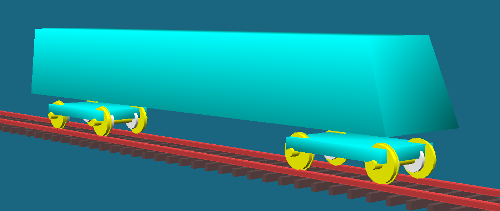
An example of a complete railway vehicle. Explanation of the input data model can be found in "Description of a rail road vehicle model". Which can be found under Rail Road applications.

Bo'Bo' is the denotation of the axle arrangement classification according to UIC (also known as German classification). For further information please see: Wikipedia. The denotation Bo'Bo' means there are two bogies under the unit and each bogie has two powered axles individually driven by traction motors. This axle arrangment is today the most common arrangement in modern locomotives.

The connection between wheels and rails can be modeled in many different ways. In this tutorial func wr_coupl_pe3 has been used.

The steps 4-10 in this tutorial follows approximately the steps suggested under Debugging a vehicle model.

In step 11 the analyzis of the vehicle starts. A main interest is to check that the vehicle follows the requirements stated in UIC518 and EN14363.

Download the example

Download the tar-file intro_tutor_3_bobo_pe3.tgz
List the contents of the tar-file with "tar -tvkz -f intro_tutor_3_bobo_pe3.tgz"
Extract the contents of the tar-file with "tar -xvkz -f intro_tutor_3_bobo_pe3.tgz"

Examine the directory "intro_tutor_3_bobo_pe3"

Many file manager programs can be used to show the file contents of directory intro_tutor_3_bobo_pe3. E.g. genfile, genterm, caja, nautilus,,, etc.
The intructions in this webpage refers to the usage of the genfile file manager program. To start program genfile, click the - icon.
Input data files for program TSIM (time-domain simulation) are located in subdirectory runf.
To see the contents of subdirectory runf, double-click subdirectory runf in the Subdirectory Area. Now the contents of subdirectory runf will appear in the File Area.
Open the file runf/tang_ideal_MXDp3.tsimf by double-clicking its name and press CTRL+o or select open->op with mouse button 3

View the vehicle in program GPLOT

Program GPLOT is a graphic program showing a three dimensional view of the vehicle.
Start program GPLOT with the file runf/tang_ideal_MXDp3.tsimf by:

Double-click directory runf/ in the subdirectory text field
Double-click file runf/tang_ideal_MXDp3.tsimf in the file text field
Press the Gplot–pushbutton

In the GPLOT-window the mouse buttons are defined as:

Mouse button #1(left) zooms the model
Mouse button #2(middle) rotates the model
Mouse button #3(right) moves the model

If you zoom in to a bogie you can see that all couplings have a hot-spot. If you press the hot-spot with mouse button #1 you will get information of that specific coupling. Below is a close up of the first bogie of the vehicle:

Close the GPLOT-window, before continuing with the next section.

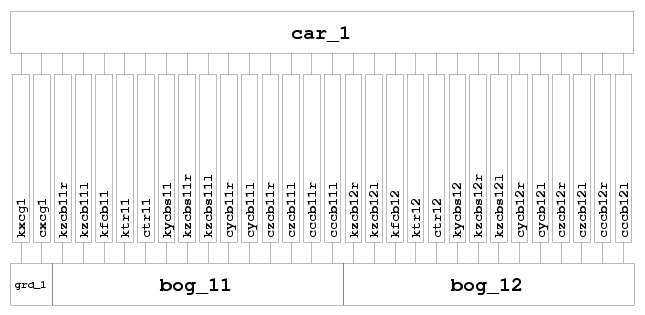
Examine the vehicle in program RUNF_INFO

Program RUNF_INFO is a program which lists how masses and couplings in the model are linked together. Program RUNF_INFO is controlled by an input data file which is described in the RUNF_INFO users manual.

Create an input data file for program RUNF_INFO
Open and examine the newly created file:
- In Subdirectory Area: double-click directory runf_infof
- In File Area double-click the runf_infof-file
- With mouse button #3 select open -> op
Execute program RUNF_INFO

Program RUNF_INFO creates the following files:

idebug/runf_info.idebug	=	Memory dump of all variables in the model
diags/runf_info.pdf	=	A two-dimensional plot, showing how all bodies connects to each other
runf_infor/tang_ideal_MXDp3.runf_infor	=	An ASCII-file containing text information about the model

Examine the files by double-clicking on them and select open->op with mouse button #3.

First diagram in diags/runf_info.pdf:

Horizontal boxes are masses.
Vertical boxes are couplings.

Close all windows except the genfile-window, before proceeding to next task.

Make a simulation on tangent track without track irregularities.

This simulation is used to check the vehicle behaves well on tangent track. Checks all masses are connected and all forces are in balance. From the genfile window perform the simulation by:

In Subdirectory Area, double-click directory runf/
In File Area, double-click file runf/tang_ideal_MXDp3.tsimf
Launch the simulation by pressing CTRL+r or with mouse button #3 select "open -> run".

Animate the simulation in program GPLOT by writing:

gplot runf/tang_ideal_MXDp3.tsimf gp/tang_ideal_MXDp3.gp &

Amplify the deformations by a factor ~200.
(You find the deformation scale factor under pulldown-menu "View -> show_1_diag")
Start animation by pressing the Fwd-button in the lower left of the GPLOT window.
As you will see the whole vehicle falls down a bit. The reason for this is that there are no prestress forces defined in the contact points between wheel and rail.
You can of course define prestress forces in the contact points, but if you later are interested in modeling sleeper irregularities you must remember to remove the prestress forces again. Otherwise the sleeper irregularities will have no effect.

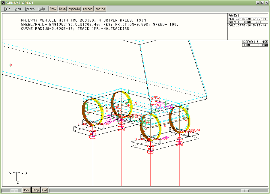
Here you can see the wheels have penetrated the rails because of the flexibility in the contact points.
(It is the very big scale factor that makes it possible to detect this deformation)

Perform a modal analysis of the vehicle

Another type analysis that is also very good to start with when debugging and getting acquainted with the model, is modal analysis.

Program MODAL calculates all possible modes of vibration in the model. Number of modes are as many as the number of equations in the model. A low damped mechanical system of one degree of freedom has two complex conjugated eigenvalues. A high damped mechanical system of one degree of freedom has two real eigenvalues, both eigenvalues are negative. A self oscillating mechanical system is a system where the real part of the eigenvalue is positive.
Before the modal analysis starts, program MODAL linearizes the nonlinear equations by an amplitude defined in command modal_param.
Make a modal analysis of the vehicle:

Copy file runf/tang_ideal_MXDp3.tsimf to runf/modalRigid_MXDp3.modalf
```
copy runf/tang_ideal_MXDp3.tsimf runf/modalRigid_MXDp3.modalf
```
Open the new file by double-clicking on runf/modalRigid_MXDp3.modalf or select open->op with the right mouse button.

If the vehicle is not in its equilibrium state, the results from program MODAL can be very wrong. Therefore it is necessary to first run program QUASI or TSIM, before program MODAL is launched. In order to do so, add a pre-process command by activating this line:

#  pre_process=  'quasi $CURRENT_FILE'

Shall be changed to:

   pre_process=  'quasi $CURRENT_FILE'

In the next step when program MODAL is launched. Read the initial values from file gp/$IDENT.gp, where $IDENT is the basename of your runf-file. This is done by activating this section:

###                                                                                                     
###     Initial values                                                                                  
#[-]{ {{{{{{{{{{{{{{{{{{{{{{{{{{{{{{{{{{{{{{{{{{{{{{{{{{{{{{{{{{{{{{{{{{{{{{{{{{{{{{{{{{{{{{{{{{{{{{{{{{
# if_then_char_init CalcType .eq. TSIM  .or.
#                   CalcType .eq. MODAL
#  initval read_gpdat gp/$IDENT.gp 1
# endif
#[-]} }}}}}}}}}}}}}}}}}}}}}}}}}}}}}}}}}}}}}}}}}}}}}}}}}}}}}}}}}}}}}}}}}}}}}}}}}}}}}}}}}}}}}}}}}}}}}}}}}}

Shall be changed to:

###                                                                                                     
###     Initial values                                                                                  
#[-]{ {{{{{{{{{{{{{{{{{{{{{{{{{{{{{{{{{{{{{{{{{{{{{{{{{{{{{{{{{{{{{{{{{{{{{{{{{{{{{{{{{{{{{{{{{{{{{{{{{{
  if_then_char_init CalcType .eq. TSIM  .or.
                    CalcType .eq. MODAL
   initval read_gpdat gp/$IDENT.gp 1
  endif
#[-]} }}}}}}}}}}}}}}}}}}}}}}}}}}}}}}}}}}}}}}}}}}}}}}}}}}}}}}}}}}}}}}}}}}}}}}}}}}}}}}}}}}}}}}}}}}}}}}}}}}

To more easily find the quasistatic position and the eigen values, make the contact patch(es) more linear. The wheel/rail-coupling func wr_coupl_pe3 is based on a piece-wise linear lookup table.
Please change these lines:

  insert file runf/wr_coupl.runf # Substructures for connecting the wheelsets to the rails.
# func char cwr_coupl=  pe3      # A lookup table for the tangential forces. Is a bit faster than pr3, but less accurate.
# func char cwr_coupl=  pe4      # Similar to pe3 but handles a varying rail profile 
  func char cwr_coupl=  pr3      # Uses Fastsim for the tangential creep forces between wheel & rail

To:

  insert file runf/wr_coupl.runf # Substructures for connecting the wheelsets to the rails.
  func char cwr_coupl=  pe3      # A lookup table for the tangential forces. Is a bit faster than pr3, but less accurate.
# func char cwr_coupl=  pe4      # Similar to pe3 but handles a varying rail profile 
# func char cwr_coupl=  pr3      # Uses Fastsim for the tangential creep forces between wheel & rail

In order to be able to see the bogie kinematic mode. Increase the vehicle speed to 300 [km/h]. Please change this line:
```
  func const vkmh= 160                          # Speed in km/h
```
To:
```
  func const vkmh= 300                          # Speed in km/h
```
Press CTRL+S to save the file
Launch program MODAL by clicking Gensys -> Run Current File in the pulldown menu.

In the output from program MODAL you can see that a number of files has been created:

id/modalRigid_MXDp3.id	MPdat -file for plotting in MPLOT
gp/modalRigid_MXDp3.gp	GPdat -file for animation in GPLOT
calcmod/modalRigid_MXDp3.mode	mode -file containing all eigenvalues
calcmod/modalRigid_MXDp3.modf	modf -file containing all eigen forms
calcmod/modalRigid_MXDp3.modjac	modjac-file for linear analysis

Open a file by double-clicking the file and select open->op with the right mouse button.
N.B. File id/modalRigid_MXDp3.id is an unformatted file and cannot be opened in a text editor. To see its contents please select open->run instead. Then program mp2ascii will open the file instead. In a popup-menu you will be able to choose what kind of output you are interested in.
Start program GPLOT, by double-clicking file runf/modalRigid_MXDp3.modalf and press the Gplot–pushbutton.
- To read the eigenvalues and modal shapes into program GPLOT, select File->read_gpdat from the pulldown menu. Double-click file gp/modalRigid_MXDp3.gp.
- When program GPLOT has read the file gp/modalRigid_MXDp3.gp, a picture of mode #1 will be shown.
- Click on Deform->draw_deform in the pulldown menu, in order to see a list of all available eigen modes.
- Double-click a mode of vibration having a relative damping less than 100%.
- Many modes are highly damped. If the damping of the mode exceeds 100% the mode does not have a harmonic solution, instead the solution is exponential.
- Eigen modes having a relative damping less than 100% are complex valued eigen modes. Each complex valued eigen modes consists of two complex conjugated value pairs. Where one of the modes has a positive eigenfrequency and the other has a negative eigenfrequency.
  In the Deform->draw_deform–menu only modes with a positive eigenfrequency has been listed. Modes of vibration having a negative eigenfrequency has been removed.
- Start animation by pressing the Fwd–pushbutton
- Eigenmodes can also be changed with the Next and Prev pushbuttons in the pull-down menu.
An alternative way of starting program GPLOT with the modalRigid-model is to write the following command:
```
gplot runf/modalRigid_MXDp3.modalf gp/modalRigid_MXDp3.gp &
```
Now both files are read into GPLOT during its startup phase.

Show animation of the lower sway mode of the BoBo-vehicle:

How to calculate the eigen modes of a mechanical system is shown in the Theory manual

Exercise:

Find the following mode shapes in the vehicle:

Lower sway:
Upper sway:
Body bounce:
Body pitch:
Body yaw:
1:st bogie kinematic mode:
2:d bogie kinematic mode:
Bogie longitudinal vibration:

Answers

Close the GPLOT-window, before continuing with the next section.

Perform a modal analysis taking car-body structural flexibility into account

Results from a modal analysis in a FEM-program of a car-body at free-free conditions are stored in the subdirectory patranr. This example shows how to take car-body structural flexibility into account:

Copy file runf/modalRigid_MXDp3.modalf to runf/modalFlex_MXDp3.modalf
```
copy runf/modalRigid_MXDp3.modalf runf/modalFlex_MXDp3.modalf
```
(If you not have the runf/modalRigid_MXDp3.modalf-file, please go to section Perform a modal analysis of the vehicle)
Double-click file runf/modalFlex_MXDp3.modalf or select open->op with the right mouse button.

Add flexible mode shapes by running program NPICK in a pre_process, before the modal analysis takes place. This is done by activating these two lines in the runf-file:

#  pre_process=  'sed "s!runf/tang_ideal_MXDp3.tsimf!$CURRENT_FILE!" npickf/flex_car.npickf > npickf/$IDENT.npickf'
#  pre_process=  'npick npickf/$IDENT.npickf'

Change them to:

   pre_process=  'sed "s!runf/tang_ideal_MXDp3.tsimf!$CURRENT_FILE!" npickf/flex_car.npickf > npickf/$IDENT.npickf'
   pre_process=  'npick npickf/$IDENT.npickf'

The results from program NPICK must also be entered into the model. This is done by activating this section in the runf-file:

###                                                                                                     
###     Flexible masses                                                                                 
#[-]{ {{{{{{{{{{{{{{{{{{{{{{{{{{{{{{{{{{{{{{{{{{{{{{{{{{{{{{{{{{{{{{{{{{{{{{{{{{{{{{{{{{{{{{{{{{{{{{{{{{
# if_then_char_init CalcType .ne. NPICK
#  insert file npickr/$IDENT.npickr
#  insert file npickr/tors.npickr       # Torsional eigenmode wheelset
# endif
#[-]} }}}}}}}}}}}}}}}}}}}}}}}}}}}}}}}}}}}}}}}}}}}}}}}}}}}}}}}}}}}}}}}}}}}}}}}}}}}}}}}}}}}}}}}}}}}}}}}}}}

The above section shall be changed to:

###                                                                                                     
###     Flexible masses                                                                                 
#[-]{ {{{{{{{{{{{{{{{{{{{{{{{{{{{{{{{{{{{{{{{{{{{{{{{{{{{{{{{{{{{{{{{{{{{{{{{{{{{{{{{{{{{{{{{{{{{{{{{{{{
  if_then_char_init CalcType .ne. NPICK
   insert file npickr/$IDENT.npickr
#  insert file npickr/tors.npickr       # Torsional eigenmode wheelset
  endif
#[-]} }}}}}}}}}}}}}}}}}}}}}}}}}}}}}}}}}}}}}}}}}}}}}}}}}}}}}}}}}}}}}}}}}}}}}}}}}}}}}}}}}}}}}}}}}}}}}}}}}}

Press CTRL+S to save the file
Launch program MODAL by clicking Gensys -> Run Current File in the pulldown menu. Program NPICK and QUASI will now automatically be executed within MODAL.
If you open file calcmod/modalFlex_MXDp3.mode and compare its contents with file calcmod/modalRigid_MXDp3.mode, you can see that we now have got 6 more eigen modes. Since each equation of motion is a second order differential equation, it will lead to two new equations for each degree of freedom. The 6 new equations are named car_1.c1, car_1.c2, car_1.c3, car_1.v1, car_1.v2 and car_1.v3. Equation car_1.c1 tells us how much the first bending mode of the car-body is excited. Equation car_1.c2 tells us how much the torsional mode of the car-body is excited. Equation car_1.c3 tells us how much the second bending mode of the car-body is excited. The equations car_1.v1, car_1.v2 and car_1.v3 tells us the speed of the first bending mode, torsional mode and second bending mode, respectively.
Start the GPLOT program, by writing:
```
gplot runf/modalFlex_MXDp3.modalf gp/modalFlex_MXDp3.gp &
```
- In order to change eigenmode: click on Deform->draw_deform in the pulldown menu or press the Next–pushbutton in the pull-down menu.
- In order to start the animation, press the Fwd–pushbutton in the lower left corner of the window.

Show animation of the first bending mode of the car-body:

If you open the Deform->draw_deform popup menu. You will see that you have got 6 more eigenvalues, compared to the previous case modalRigid. These new equations arise from the three flexible modes added by program NPICK.

Exercise:

Find the following mode shapes in the vehicle:

Lower sway:
Upper sway:
Body bounce:
Body pitch:
Body yaw:
1:st bogie kinematic mode:
2:d bogie kinematic mode:
Car-body bending mode in phase with bogies:
Car-body bending mode out of phase with bogies:
Car-body torsion mode:
Car-body 2:d bending mode:

Answers

Please close the GPLOT-window, before continuing with the next section.

Modal analysis if program QUASI struggles in finding a quasi-static position

There are many reasons why program QUASI sometimes can have difficulties to find the quasi-static position of the vehicle. If this happens, there is a possibility to use program TSIM instead. In order to use program TSIM do the following:

Copy file runf/tang_ideal_MXDp3.tsimf to runf/tang_ideal_MXDp3_vkmh300.tsimf
```
copy runf/tang_ideal_MXDp3.tsimf runf/tang_ideal_MXDp3_vkmh300.tsimf
```

Change line from:

  func const vkmh= 160                          # Speed in km/h

To:

  func const vkmh= 300                          # Speed in km/h

Press CTRL+S to save file runf/tang_ideal_MXDp3_vkmh300.tsimf
Launch program TSIM by clicking Gensys -> Run Current File in the pulldown menu.
To check that the simulation is long enough to find the quasi-static position. Please start program MPLOT and look at the wheel/rail contact forces. In the end of the simulation, no vibrations should remain.
If all curves ends without vibrations. The last timestep can be considered as the quasi-static position of the vehicle. Then proceed and make the modal analysis using this position as initial value.
Copy file runf/tang_ideal_MXDp3_vkmh300.tsimf to runf/modalRigid_MXDp3_tsim.modalf
```
copy runf/tang_ideal_MXDp3_vkmh300.tsimf runf/modalRigid_MXDp3_tsim.modalf
```

Open file runf/modalRigid_MXDp3_tsim.modalf and change the following lines:

###                                                                                                     
###     Initial values                                                                                  
#[-]{ {{{{{{{{{{{{{{{{{{{{{{{{{{{{{{{{{{{{{{{{{{{{{{{{{{{{{{{{{{{{{{{{{{{{{{{{{{{{{{{{{{{{{{{{{{{{{{{{{{
# if_then_char_init CalcType .eq. TSIM  .or.
#                   CalcType .eq. MODAL
#  initval read_gpdat gp/$IDENT.gp 1
# endif
#[-]} }}}}}}}}}}}}}}}}}}}}}}}}}}}}}}}}}}}}}}}}}}}}}}}}}}}}}}}}}}}}}}}}}}}}}}}}}}}}}}}}}}}}}}}}}}}}}}}}}}

To:

###                                                                                                     
###     Initial values                                                                                  
#[-]{ {{{{{{{{{{{{{{{{{{{{{{{{{{{{{{{{{{{{{{{{{{{{{{{{{{{{{{{{{{{{{{{{{{{{{{{{{{{{{{{{{{{{{{{{{{{{{{{{{{
  if_then_char_init CalcType .eq. TSIM  .or.
                    CalcType .eq. MODAL
   initval read_gpdat gp/tang_ideal_MXDp3_vkmh300.gp -1
  endif
#[-]} }}}}}}}}}}}}}}}}}}}}}}}}}}}}}}}}}}}}}}}}}}}}}}}}}}}}}}}}}}}}}}}}}}}}}}}}}}}}}}}}}}}}}}}}}}}}}}}}}}

Deformation state number "-1", refers to the last deformation state in the .gp-file.
Press CTRL+S to save file runf/modalRigid_MXDp3_tsim.modalf
Launch program MODAL by clicking Gensys -> Run Current File in the pulldown menu.

Find the non-linear critical speed of the vehicle.

Copy file runf/tang_ideal_MXDp3.tsimf to runf/crit_ideal_MXDp3.tsimf
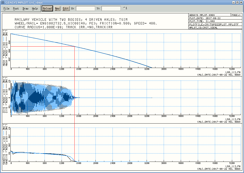
```
copy runf/tang_ideal_MXDp3.tsimf runf/crit_ideal_MXDp3.tsimf
```

Open file runf/crit_ideal_MXDp3.tsimf and change the lines from:

  func const knwr_= 600e6        # Wheel/rail normal contact stiffness
  func const mu_  = 0.36         # Friction between wheel and rail
# func const mulf_= 1.           # Kalker factor (if undefined, runf/wr_coupl.runf will set mulf_= mu_/0.6)

to:

  func const knwr_= 600e6        # Wheel/rail normal contact stiffness
  func const mu_  = 0.50         # Friction between wheel and rail
  func const mulf_= 1.           # Kalker factor (if undefined, runf/wr_coupl.runf will set mulf_= mu_/0.6)

Change the lines from:

#
  func const vkmh= 160                          # Speed in km/h
#
# func const vkmh_deacc=  5                     # Retardation of the train-set, when calculating critical speed
# func operp vkmh= 440 - vkmh_deacc * time      # Vary vkmh linearily

to:

#
# func const vkmh= 160                          # Speed in km/h
#
  func const vkmh_deacc=  5                     # Retardation of the train-set, when calculating critical speed
  func operp vkmh= 440 - vkmh_deacc * time      # Vary vkmh linearily

Change the lines from:

###                                                                                                     
###     Excite and reduce the vehicle speed, to calculate critical speed                                
#[-]{ {{{{{{{{{{{{{{{{{{{{{{{{{{{{{{{{{{{{{{{{{{{{{{{{{{{{{{{{{{{{{{{{{{{{{{{{{{{{{{{{{{{{{{{{{{{{{{{{{{
#
# force rel_lsys1  deacc_car_1  car_1  0 0 -hccg_1 -mc_1*vkmh_deacc*1000/3600  0. 0.  0. 0. 0.  # Apply negative longitudinal forces,
# in_substruct crit_excit   [ 11 ]   # $1= bog_no                                               # to create the retardation "vkmh_deacc".
# in_substruct crit_excit   [ 12 ]                                                              # (The unit of "vkmh_deacc" is [km/h/s])
#

to:

###                                                                                                     
###     Excite and reduce the vehicle speed, to calculate critical speed                                
#[-]{ {{{{{{{{{{{{{{{{{{{{{{{{{{{{{{{{{{{{{{{{{{{{{{{{{{{{{{{{{{{{{{{{{{{{{{{{{{{{{{{{{{{{{{{{{{{{{{{{{{
#
  force rel_lsys1  deacc_car_1  car_1  0 0 -hccg_1 -mc_1*vkmh_deacc*1000/3600  0. 0.  0. 0. 0.  # Apply negative longitudinal forces,
  in_substruct crit_excit   [ 11 ]   # $1= bog_no                                               # to create the retardation "vkmh_deacc".
  in_substruct crit_excit   [ 12 ]                                                              # (The unit of "vkmh_deacc" is [km/h/s])
#

(To easily remove all comment signs "#". Mark all lines and press CTRL+3)

Change the line from:

  tstop=  10.

to:

  tstop=  25.

Press CTRL+S to save the file
Launch program TSIM by clicking Gensys -> Run Current File in the pulldown menu.
Double-click the file mplotf/critSpeedPlot.mplotf in the mplotf-directory.
Launch program MPLOT by pressing Ctrl+R. Select ident crit_ideal
Estimate the critical speed in the plot. In order to make the estimate more accurate, use the middle mouse button. When the middle mouse button is pressed the position of the mouse can seen in the text fields at the top of the window.
Calculate the critical speed defined as max.track-shift force less than 2.5[kN], by running script ./crit_bobo.sh
Output:
```
Ident               Critical speed
-----------------------------------
crit_ideal_MXDp3	374.545400
```

Make a simulation through a curve, without track irregularities.

Copy file runf/tang_ideal_MXDp3.tsimf to runf/R600_ideal_MXDp3.tsimf
```
copy runf/tang_ideal_MXDp3.tsimf runf/R600_ideal_MXDp3.tsimf
```

Open file runf/R600_ideal_MXDp3.tsimf and change the lines from:

  func const CurveRadius=  1e99                 # Curve radius in [m]
  func const CurveCant=   0.000                 # Cant of track in [m]

to:

  func const CurveRadius=   600                 # Curve radius in [m]
  func const CurveCant=   0.150                 # Cant of track in [m]

Change lines from:

# func const vkmh= 3.6*sqrt(CurveRadius*(Y_cp+CurveCant/(2*bo_)*9.81))
# no_warning func min vkmh= vkmh 160
#
  func const vkmh= 160                          # Speed in km/h

to:

  func const vkmh= 3.6*sqrt(CurveRadius*(Y_cp+CurveCant/(2*bo_)*9.81))
  no_warning func min vkmh= vkmh 160
#
# func const vkmh= 160                          # Speed in km/h

(The speed vkmh will be automatically calculated giving a uncompensated lateral acceleration of 0.6540[m/s²] in the track plane)

Change line from:
```
  tstop=  10.
```
to:
```
  tstop=  25.
```
Press CTRL+S to save the file
Launch program TSIM by clicking Gensys -> Run Current File in the pulldown menu.
Animate the results in GPLOT by writing:
```
gplot runf/R600_ideal_MXDp3.tsimf gp/R600_ideal_MXDp3.gp &
```
- Set the Deformation scale fact equal to 10 approximately
- Animate Contact forces by selecting View->show_4_diags from the pulldown menu
Show animation in GPLOT:

Animate the results in GLPLOT by writing:

glplot runf/R600_ideal_MXDp3.tsimf gp/R600_ideal_MXDp3.gp &

Show animation in GLPLOT:
Display the results in MPLOT.
Double-click the mplotf/-directory. Double-click the mplotf/Tsim_All_BoBo.mplotf-file in the right window. Select open->run with the right mouse button. In the MPLOT command line popup menu select ident R600_ideal_MXDp3.
In file mplotf/Tsim_All_BoBo.mplotf a number of plots are predefined, you can select plot with the radio-buttons to the right of the pulldown menu bar. The predefined plots are shown here:

Make a simulation through a curve, with track irregularities and in-line post processing.

Copy file runf/R600_ideal_MXDp3.tsimf to runf/R600_tirr_MXDp3.tsimf
```
copy runf/R600_ideal_MXDp3.tsimf runf/R600_tirr_MXDp3.tsimf
```

Open file runf/R600_tirr_MXDp3.tsimf and change line from:

#  post_process= 'mplot mplotf/Tsim_All_BoBo.mplotf $IDENT'

to:

   post_process= 'mplot mplotf/Tsim_All_BoBo.mplotf $IDENT'

Change line from:

  func char  ctrack_irreg=  Ideal_track         # Output in header lines

to:

  func char  ctrack_irreg=  track_V120a         # Output in header lines

Press CTRL+S to save the file
Launch program TSIM by clicking Gensys -> Run Current File in the pulldown menu.

Inspect the results from post processor MPLOT.
In the end of the simulation you can see that three result files were generated mplotr/R600_tirr_MXDp3.print, diags/R600_tirr_MXDp3.ps and mplotr/R600_tirr_MXDp3.resu. The files have the following contents:

mplotr/R600_tirr_MXDp3.print
Output of scalars defined in command print in the file mplotf/Tsim_All_BoBo.mplotf. In current example the file has the following contents:

car_1.m.Nmv	Mean Comfort simplified according to CEN Technical
car_1b1.Nmv	Committee 256 WG 7 and ERRI Question B 153.
car_1b2.Nmv	At center of car-body, over bogie #1 and over bogie #2 respectively.
S1_max	Max lateral track-shift force
Y/Q_1_max	Max flange climb ratio
bt1MIN	Min vehicle turnover ratio
car_1b2.yMAX	Max pantograph sway over trailing bogie
car_1b2.yMIN	Min pantograph sway over trailing bogie

diags/R600_tirr_MXDp3.ps
Plots written in postscript format.
mplotr/R600_tirr_MXDp3.resu
Result summaries from all FTWZ- and STAT- commands given in the mplotf/Tsim_All_BoBo.mplotf-file.

Open and inspect the results by double-clicking the files and select open->op with the right mouse button.

Estimate average wear over a longer track section. Method #1

The simplest method to estimate the wear on wheels and rails, is to calculate the quasi-static portion of the dissipated energy in the contact points. Track irregularities also contribute to wear, but the main portion of the wear is quasi-static due to the curve geometry. To perform this task use program OPTI to initiate several simulations, one simulation for each curve radius.

First create an input data file for program TSIM:

Copy file runf/tang_ideal_MXDp3.tsimf into runf/wear_curve_MXDp3.tsimf.
```
copy runf/tang_ideal_MXDp3.tsimf runf/wear_curve_MXDp3.tsimf
```
Open file runf/wear_curve_MXDp3.tsimf
Run program MPLOT through a post-process command. The last value of the simulation is considered as being the quasi-static value.
Change:
```
#  post_process= 'mplot mplotf/wear_curve_scal.mplotf   $IDENT'
```
To:
```
   post_process= 'mplot mplotf/wear_curve_scal.mplotf   $IDENT'
```

Run in right handed curves.
Change:

###                                                                                                     
###     Designed(nominal) track geometry                                                                
###  -------------------------------------------------------------                                      
  func const CurveRadius=  1e99                # Curve radius in [m]
  func const CurveCant=   0.000                # Cant of track in [m]
#[-]{ {{{{{{{{{{{{{{{{{{{{{{{{{{{{{{{{{{{{{{{{{{{{{{{{{{{{{{{{{{{{{{{{{{{{{{{{{{{{{{{{{{{{{{{{{{{{{{{{{{
#
  func intpl_r ro_trac_design  -100.+Xtrac_start  0.
                                 50.+Xtrac_start  0.
                                150.+Xtrac_start  1/CurveRadius         # Right handed curve
                                200.+Xtrac_start  1/CurveRadius
                                300.+Xtrac_start  0.
                                350.+Xtrac_start  0.
                                450.+Xtrac_start -1/CurveRadius         # Left handed curve
                                500.+Xtrac_start -1/CurveRadius
                                600.+Xtrac_start  0.
                              10000.+Xtrac_start  0.
  func intpl_r f_trac_design   -100.+Xtrac_start  0.
                                 50.+Xtrac_start  0.
                                150.+Xtrac_start  CurveCant/(2*bo_)
                                200.+Xtrac_start  CurveCant/(2*bo_)
                                300.+Xtrac_start  0.
                                350.+Xtrac_start  0.
                                450.+Xtrac_start -CurveCant/(2*bo_)
                                500.+Xtrac_start -CurveCant/(2*bo_)
                                600.+Xtrac_start  0.
                              10000.+Xtrac_start  0.
  func intpl_r z_trac_design   -100.+Xtrac_start  0.
                                 50.+Xtrac_start  0.
                                150.+Xtrac_start -abs(CurveCant)/2.
                                200.+Xtrac_start -abs(CurveCant)/2.
                                300.+Xtrac_start  0.
                                350.+Xtrac_start  0.
                                450.+Xtrac_start -abs(CurveCant)/2.
                                500.+Xtrac_start -abs(CurveCant)/2.
                                600.+Xtrac_start  0.
                              10000.+Xtrac_start  0.

To:

###                                                                                                     
###     Designed(nominal) track geometry                                                                
###  -------------------------------------------------------------                                      
  func const CurveRadius=  1e99                # Curve radius in [m]
  func const CurveCant=   0.000                # Cant of track in [m]
#[-]{ {{{{{{{{{{{{{{{{{{{{{{{{{{{{{{{{{{{{{{{{{{{{{{{{{{{{{{{{{{{{{{{{{{{{{{{{{{{{{{{{{{{{{{{{{{{{{{{{{{
#
  func intpl_r ro_trac_design  -100.+Xtrac_start  0.
                                 50.+Xtrac_start  0.
                                150.+Xtrac_start  1/CurveRadius         # Right handed curve
                              10000.+Xtrac_start  1/CurveRadius
  func intpl_r f_trac_design   -100.+Xtrac_start  0.
                                 50.+Xtrac_start  0.
                                150.+Xtrac_start  CurveCant/(2*bo_)
                              10000.+Xtrac_start  CurveCant/(2*bo_)
  func intpl_r z_trac_design   -100.+Xtrac_start  0.
                                 50.+Xtrac_start  0.
                                150.+Xtrac_start -abs(CurveCant)/2.
                              10000.+Xtrac_start -abs(CurveCant)/2.

Set the speed in order to get a constant cant deficiency for all curves: (max speed= 160 km/h)
Change:

# func const vkmh= 3.6*sqrt(CurveRadius*(Y_cp+CurveCant/(2*bo_)*9.81))
# no_warning func min vkmh= vkmh 160
#
  func const vkmh= 160                          # Speed in km/h

To:

  func const vkmh= 3.6*sqrt(CurveRadius*(Y_cp+CurveCant/(2*bo_)*9.81))
  no_warning func min vkmh= vkmh 160
#
# func const vkmh= 160                          # Speed in km/h

Change the simulation time from:
```
  tstop=  10.
```
to:
```
  tstop=  25.
```
Open file optif/wear_curve.optif and check which simulation cases has been defined.
Launch the simulations by double-click file optif/wear_curve.optif and select open -> run with mouse button 3.
Check the status of the jobs by clicking "Start -> Queue monitor" in the GENFILE pulldown menu.
If the calculations in SLURM do not start, please consult section Debugging SLURM.
Wait until all calculations are finished.
Run input data file mplotf/wear_curve_scal_plot.mplotf. The file will create a curve of wear v.s. curve radius.
Example:

When running file mplotf/wear_curve_scal_plot.mplotf it is not necessary to give an ident in the startup menu window, because all idents are defined in the file.
On the question MPdat-file "mplot_id.mp" exists answer Replace or Use, it doesn't matter, because the mplot_id-ident is empty.

Alternatively run input data file mtablef/wear_curve_scal.mtablef. Program MTABLE will collect all results from all calculations and present the summary in a table.

#
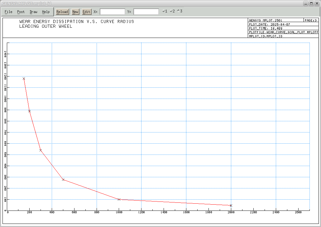
#                           |CurveRadius|       vkmh|cpa_111l.FM|cpa_111r.FM|cpa_111l.Fn|cpa_111r.Fn| 
#                           |           |           |    nu_scal|    nu_scal|     u_scal|     u_scal| 
#Date:      Idents:         |           |           |           |           |           |           | Head lines:
#                           |         1.|         1.|         1.|         1.|         1.|         1.|
#-------------------------------------------------------------------------------------------------------------------------------------------------------------------------------------
2025-04-07  wear_curve_00001     150.000      56.378    1181.480     436.236    1151.078     436.178  Wheel/Rail= ENS1002t32.5_60E1i40; pr3; Friction=.36; Speed=56.38
2025-04-07  wear_curve_00002     200.000      65.099     888.768     363.557     854.044     363.482  Wheel/Rail= ENS1002t32.5_60E1i40; pr3; Friction=.36; Speed=65.1
2025-04-07  wear_curve_00003     300.000      79.730     538.622     259.765     502.788     259.655  Wheel/Rail= ENS1002t32.5_60E1i40; pr3; Friction=.36; Speed=79.73
2025-04-07  wear_curve_00004     500.000     102.931     276.228     153.916     261.477     153.715  Wheel/Rail= ENS1002t32.5_60E1i40; pr3; Friction=.36; Speed=102.9
2025-04-07  wear_curve_00005    1000.000     142.625      98.250      72.352     100.705      72.195  Wheel/Rail= ENS1002t32.5_60E1i40; pr3; Friction=.36; Speed=142.6
2025-04-07  wear_curve_00006    2000.000     160.000      44.650      20.003      41.770      19.922  Wheel/Rail= ENS1002t32.5_60E1i40; pr3; Friction=.36; Speed=160

The two largest values in each column are marked with a red color. The two smallest values in each column are marked with a blue color. In program MTABLE limit values can be defined, values over the limit will be marked with a red bold font.

Calculate the curve radius distribution of the track.
Example:

Multiply each bar in the histogram with the wear distribution, and a total average wear can be estimated.

#
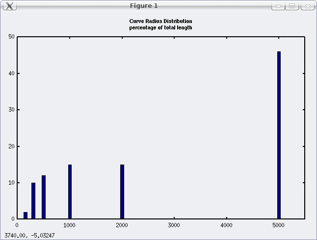
# Average energy dissipation, left and right side, wheelset 111
# -------------------------------------------------------------
 genoctave2 "(1181.479 + 436.237) / 2."= 808.86        ;# R=  150[m]
 genoctave2 "( 888.769 + 363.558) / 2."= 626.16        ;# R=  200[m]
 genoctave2 "( 538.623 + 259.765) / 2."= 399.19        ;# R=  300[m]
 genoctave2 "( 276.228 + 153.916) / 2."= 215.07        ;# R=  500[m]
 genoctave2 "(  98.250 +  72.352) / 2."=  85.30        ;# R= 1000[m]
 genoctave2 "(  44.650 +  20.003) / 2."=  32.33        ;# R= 2000[m]

#
# Track curve distribution
# ------------------------
#  R150= 0.02
#  R200= 0.01
#  R300= 0.10
#  R500= 0.12
# R1000= 0.15
# R2000= 0.15

#
# Total average energy dissipation, wheelset 111, running on above track curve distribution
# -----------------------------------------------------------------------------------------
#             R= 150       R= 200       R= 300       R= 500       R= 1000      R= 2000
 genoctave2 ".02*808.86 + .01*626.16 + .10*399.19 + .12*215.07 + .15*85.30 + .15*32.33"= 106

I.e. the average wear over the whole track section is

106 [J/m]

If you want to add more curve radiuses in the wear v.s. curve radius plot:
- Open file optif/wear_curve.optif
- Add more cases under runf_subst
- Rerun file optif/wear_curve.optif with option Overwrite set equal to Append.
- Do not change anything under runf_text, otherwise option Append cannot be used.

Estimate average wear over a longer track section. Method #2

This method requires more calculation, but gives more and better results. In this method all steps in the wear loop are performed with the octave script wear_loop.m. The script makes the following calculations in each step:

Calculates wheel/rail geometry functions
Makes a simulation over the whole track section
Calculates the wear depth on the different places on the wheel profile
Removes material from the wheel profile

With this method it is possible to see if the wear will lead to thicker or thinner flanges.

To execute this example:

Go to directory wear_loop by writing
```
cd wear_loop
```
Double-click file wear_loop.m and select open -> run with the right mouse button
All wheel profiles from all wear steps can be found under directory kpf/w_prof
The wheel profiles can be plotted with script wear_loop_plot.m. Double-click file wear_loop_plot.m and select open -> run with the right mouse button.

Modeling of wheel flange lubrication.

Copy file runf/R600_ideal_MXDp3.tsimf to runf/R600_ideal_MXDp3_wheel_lubr.tsimf
```
copy runf/R600_ideal_MXDp3.tsimf runf/R600_ideal_MXDp3_wheel_lubr.tsimf
```
Open file runf/R600_ideal_MXDp3_wheel_lubr.tsimf

Change head 3 from

  head 3 "Wheel/Rail= $ckpfr; $cwr_coupl; Friction=$mu_; Speed=$vkmh"

  head 3 "Wheel/Rail= $ckpfr; $cwr_coupl; Friction=$muTread $muFlange; Speed=$vkmh"

Under "Wheel-rail contact model"
Change the friction coefficient from:

  func const knwr_= 600e6        # Wheel/rail normal contact stiffness
  func const mu_  = 0.36         # Friction between wheel and rail
# func const mulf_= 1.           # Kalker factor (if undefined, runf/wr_coupl.runf will set mulf_= mu_/0.6)

to:

  func const knwr_= 600e6        # Wheel/rail normal contact stiffness
# func const mu_  = 0.36         # Friction between wheel and rail
# func const mulf_= 1.           # Kalker factor (if undefined, runf/wr_coupl.runf will set mulf_= mu_/0.6)

##
##      Friction coefficients individual for each contact patch on all wheels
##      (will later be adjusted by substruct update_wheel_mu)
##      ==========================================================================================
  func const   muTread = 0.5    # Friction coeff on tread
  func const   muFlange= 0.1    # Friction coeff on flange

Create individual friction coefficients for all patches, by activating the following line:

##                                                                                                      
##      Create individual variables for all friction coefficients                                       
##     (will later be adjusted by substruct update_wheel_mu and/or update_rail_mu)                      
##      ==========================================================================================      
# in_substruct create_mu [ $1 ]                          # $1= axl_no

change to:

##                                                                                                      
##      Create individual variables for all friction coefficients                                       
##     (will later be adjusted by substruct update_wheel_mu and/or update_rail_mu)                      
##      ==========================================================================================      
  in_substruct create_mu [ $1 ]                          # $1= axl_no

Update the friction coefficients depending on the location of the contact patches, by activating the following line:

##                                                                                                      
##      Update the friction coeff depending on the location of the contact patch. Wheel lubrication     
##      ===========================================================================================     
# in_substruct update_wheel_mu  [ $1 ]                   # $1= axl_no

change to:

##                                                                                                      
##      Update the friction coeff depending on the location of the contact patch. Wheel lubrication     
##      ===========================================================================================     
  in_substruct update_wheel_mu  [ $1 ]                   # $1= axl_no

Press CTRL+S to save the file
Launch program TSIM by clicking Gensys -> Run Current File in the pulldown menu.
Compare the results with the results obtained under Make a simulation through a curve, without track irregularities.

Modeling of rail lubrication.

Copy file runf/R600_ideal_MXDp3.tsimf to runf/R600_ideal_MXDp3_rail_lubr.tsimf
```
copy runf/R600_ideal_MXDp3.tsimf runf/R600_ideal_MXDp3_rail_lubr.tsimf
```
Open file runf/R600_ideal_MXDp3_rail_lubr.tsimf

Change the header lines from:

  head 2 "Railway vehicle with two bogies; 4 driven axles; $CalcType"
  head 3 "Wheel/Rail= $ckpfr; $cwr_coupl; Friction=$mu_; Speed=$vkmh"
  head 4 "Curve Radius=$CurveRadius; Track irr.=$ctrack_irreg"

  head 2 "Railway vehicle with two bogies; 4 driven axles; $CalcType"
  head 3 "Wheel/Rail= $ckpfr;                              Speed=$vkmh"
  head 4 "Curve Radius=$CurveRadius; Track irr.=$ctrack_irreg"
  head 5 "Friction mu_def=$mu_def mu_or=$mu_or mu_ir=$mu_ir mu_gcor=$mu_gcor"

Under "Wheel-rail contact model"
Change the friction coefficient from:

  func const knwr_= 600e6        # Wheel/rail normal contact stiffness
  func const mu_  = 0.36         # Friction between wheel and rail
# func const mulf_= 1.           # Kalker factor (if undefined, runf/wr_coupl.runf will set mulf_= mu_/0.6)

to:

  func const knwr_= 600e6        # Wheel/rail normal contact stiffness
# func const mu_  = 0.36         # Friction between wheel and rail
# func const mulf_= 1.           # Kalker factor (if undefined, runf/wr_coupl.runf will set mulf_= mu_/0.6)

##
## Friction coefficient. Rail lubrication
## ----------------------------------------------
  func const mu_radius= 1/750  # Lubricate all curves tighter than 750 m                        
  func const   mu_def = 0.5    # Default friction coeff valid for curves bigger than 750 m      
  func const   mu_or  = 0.5    # Default friction coeff in curves; outer rail                   
  func const   mu_ir  = 0.25   # Default friction coeff in curves; inner rail                   
  func const   mu_gcor= 0.1    # Friction coeff on gauge corner and below; outer rail

Create individual friction coefficients for all patches, by activating the following line:

##                                                                                                      
##      Create individual variables for all friction coefficients                                       
##     (will later be adjusted by substruct update_wheel_mu or update_rail_mu)                          
##      ==========================================================================================      
# in_substruct create_mu [ $1 ]                          # $1= axl_no

change to:

##                                                                                                      
##      Create individual variables for all friction coefficients                                       
##     (will later be adjusted by substruct update_wheel_mu or update_rail_mu)                          
##      ==========================================================================================      
  in_substruct create_mu [ $1 ]                          # $1= axl_no

Update the friction coefficients depending on the location of the contact patches, by activating the following line:

##                                                                                                      
##      Update the friction coeff depending on the location of the contact patch. Rail lubrication      
##      ===========================================================================================     
# in_substruct update_rail_mu  [ $1  ]                   # $1= axl_no

change to:

##                                                                                                      
##      Update the friction coeff depending on the location of the contact patch. Rail lubrication      
##      ===========================================================================================     
  in_substruct update_rail_mu  [ $1  ]                   # $1= axl_no

Press CTRL+S to save the file
Launch program TSIM by clicking Gensys -> Run Current File in the pulldown menu.
Compare the results with the results obtained under Make a simulation through a curve, without track irregularities.

Modeling of individually rotating wheels.

Critical speed:

Copy file runf/tang_ideal_IRW.tsimf to runf/crit_ideal_IRW.tsimf
```
copy runf/tang_ideal_IRW.tsimf runf/crit_ideal_IRW.tsimf
```

Open file runf/crit_ideal_IRW.tsimf and change the lines from:

#
  func const vkmh= 160                          # Speed in km/h
#
# func const vkmh_deacc=  5                     # Retardation of the train-set, when calculating critical speed
# func operp vkmh= 900 - vkmh_deacc * time      # Vary vkmh linearily

to:

#
# func const vkmh= 160                          # Speed in km/h
#
  func const vkmh_deacc=  5                     # Retardation of the train-set, when calculating critical speed
  func operp vkmh= 900 - vkmh_deacc * time      # Vary vkmh linearily

Change the line from:

# force rel_lsys1  deacc_car_1  car_1  0 0 -hccg_1 -mc_1*vkmh_deacc*1000/3600  0. 0.  0. 0. 0.  # Apply negative longitudinal forces,
# in_substruct crit_excit   [ 11 ]   # $1= bog_no                                               # to create the retardation "vkmh_deacc".
# in_substruct crit_excit   [ 12 ]                                                              # (The unit of "vkmh_deacc" is [km/h/s])

to:

  force rel_lsys1  deacc_car_1  car_1  0 0 -hccg_1 -mc_1*vkmh_deacc*1000/3600  0. 0.  0. 0. 0.  # Apply negative longitudinal forces,
  in_substruct crit_excit   [ 11 ]   # $1= bog_no                                               # to create the retardation "vkmh_deacc".
  in_substruct crit_excit   [ 12 ]                                                              # (The unit of "vkmh_deacc" is [km/h/s])

Change the line from:

  tstop=  10.

to:

  tstop=  30.

Press CTRL+S to save the file
Launch program TSIM by clicking Gensys -> Run Current File in the pulldown menu.
Search for the non-linear critical speed in program MPLOT or by using script ./crit_bobo.sh

As you can see, for this vehicle the critical speed is higher ~824km/h. The critical speed depends on the moment of inertia of the wheels. If the speed is high enough, the moment of inertia of the wheels starts to make the wheelset to behave like a rigid wheelset.

Make a simulation through a curve, without track irregularities:

Copy file runf/tang_ideal_IRW.tsimf to runf/R600_ideal_IRW.tsimf
```
copy runf/tang_ideal_IRW.tsimf runf/R600_ideal_IRW.tsimf
```

Open file runf/R600_ideal_IRW.tsimf and change the line from:

#  post_process= 'mplot mplotf/Tsim_All_BoBo.mplotf $IDENT'

to:

   post_process= 'mplot mplotf/Tsim_All_BoBo.mplotf $IDENT'

Change lines from:

  func const CurveRadius=  1e99                 # Curve radius in [m]
  func const CurveCant=   0.000                 # Cant of track in [m]

to:

  func const CurveRadius=   600                 # Curve radius in [m]
  func const CurveCant=   0.150                 # Cant of track in [m]

Change lines from:

# func const vkmh= 3.6*sqrt(CurveRadius*(Y_cp+CurveCant/(2*bo_)*9.81))
# no_warning func min vkmh= vkmh 160
#
  func const vkmh= 160                          # Speed in km/h

to:

  func const vkmh= 3.6*sqrt(CurveRadius*(Y_cp+CurveCant/(2*bo_)*9.81))
  no_warning func min vkmh= vkmh 160
#
# func const vkmh= 160                          # Speed in km/h

(The speed vkmh will be automatically calculated giving a lateral acceleration of 0.6540[m/s²] in the track plane)

Change line from:
```
  tstop=  10.
```
to:
```
  tstop=  25.
```
Press CTRL+S to save the file
Launch program TSIM by clicking Gensys -> Run Current File in the pulldown menu.
Compare the results with the results obtained under Make a simulation through a curve, without track irregularities.

Passenger vehicle.

The above vehicle model describes a quite heavy motor-car approximately. If you want to study a lighter passenger-car without motors, please use runf/tang_ideal_passengerCar.tsimf as Master file.

A vehicle model with faults.

A vehicle model contains of many input data, and errors in input data may happen for different reasons. Because of that, it is important to check and debug the model before starting large scale simulations. At Debugging a vehicle model you can find some simple tips to debug the model.
Please read Debugging a vehicle model and try to find the errors in file runf/tang_ideal_err.tsimf.
(At least 3 errors should be possible to find.)

Tutorial BoBo-vehicle

Introduction

Download the example

Examine the directory "intro_tutor_3_bobo_pe3"

View the vehicle in program GPLOT

Examine the vehicle in program RUNF_INFO

Make a simulation on tangent track without track irregularities.

Perform a modal analysis of the vehicle

Perform a modal analysis taking car-body structural flexibility into account

Modal analysis if program QUASI struggles in finding a quasi-static position

Find the non-linear critical speed of the vehicle.

Make a simulation through a curve, without track irregularities.

Make a simulation through a curve, with track irregularities and in-line post processing.

Estimate average wear over a longer track section. Method #1

Estimate average wear over a longer track section. Method #2

Modeling of wheel flange lubrication.

Modeling of rail lubrication.

Modeling of individually rotating wheels.

Passenger vehicle.

A vehicle model with faults.

Tutorial
BoBo-vehicle